STARK-proving low-degree-ness of a data availability root: some analysis

This post assumes familiarity with data availability sampling as in https://arxiv.org/abs/1809.09044.

The holy grail of data availability sampling is it we could remove the need for fraud proofs to check correctness of an encoded Merkle root. This can be done with polynomial commitments (including FRI), but at a high cost: to prove the value of any specific coordinate D[i] \in D, you would need a proof that \frac{D - x}{X - i} where x is the claimed value of D[i], is a polynomial, and this proof takes linear time to generate and is either much larger (as in FRI) or relies on much heavier assumptions (as in any other scheme) than the status quo, which is a single Merkle branch.

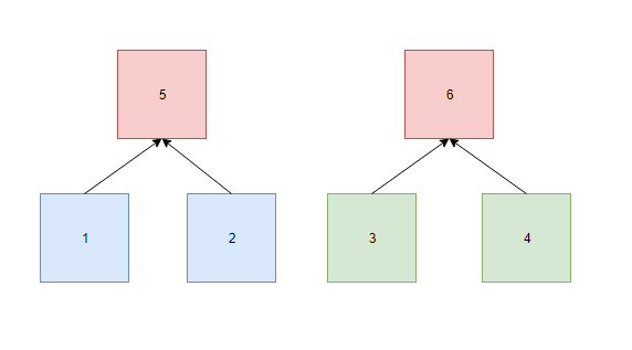
So what if we just bite the bullet and directly use a STARK (or other ZKP) to prove that a Merkle root of encoded data D[0]...D[2n-1] with degree < n is “correct”? That is, we prove that Merkle root actually is the Merkle root of data encoded in such a way, with zero mistakes. Then, data availability sampling would become much easier, a more trivial matter of randomly checking Merkle branches, knowing that if more than 50% of them are available then the rest of D can be reconstructed and it would be valid. There would be no fraud proofs and hence no network latency assumptions.

Here is a concrete construction for the arithmetic representation of the STARK that would be needed to prove this. Let us use the MIMC hash function with a sponge construction for our hash:

p = [modulus]
r = [quadratic nonresidue mod p]
k = [127 constants]

def mimc_hash(x, y):
    L, R = x, 0
    for i in range(127):
        L, R = (L**3 + 3*q*L*R**2 + k[i]) % p, (3*L**2*b + q*R**3) % p
    L = y
    for i in range(127):
        L, R = (L**3 + 3*q*L*R**2 + k[i]) % p, (3*L**2*b + q*R**3) % p
    return L

The repeated loops are cubing in a quadratic field. If desired, we can prevent analysis over Fp^2 by negating the x coordinate (ie. L) after every round; this is a permutation that is a non-arithmetic operation over Fp^2 so the function could only be analyzed as a function over Fp of two values.

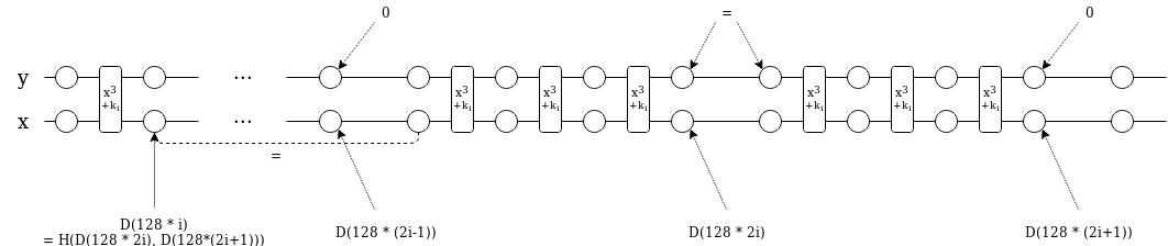
Now here is how we will set up the constraints. We position the values in D at 128 * k for 2n \le k < 4n (so x[128 * (2n + i)] = D[i]). We want to set up the constraint: x(128 * i) = H(x(128 * 2i) + x(128 * (2i+1)), at least for i < 2n; this alone would prove that x(128) is the Merkle root of D (we’ll use a separate argument to prove that D is low-degree). However, because H is a very-high-degree function, we cannot just set up that constraint directly. So here is what we do instead:

  • We have two program state values, x and y, to fit the two-item MIMC hash function.
  • For all i where i\ \%\ 128 \ne 0, we want x(i) = x(i+1)^3 + 3q*x(i+1)y(i+1)^2 + k(i) and y(i) = 3*x(i+1)^2y(i+1) + q*y(i+1)^3
  • For all i where i\ \%\ 128 = 0, we want:
    • If i < 128 * 2n, x(i) = x(2i-127)
    • If i\ \%\ 256 = 128, y(i) = y(i+1)
    • If i\ \%\ 256 = 0, y(i) = 0

[Edit 2019.10.09: some have argued that for technical reasons the x(i) = x(2i-127) constraint cannot be soundly enforced. If this is the case, we can replace it with a PLONK-style coordinate-accumulator-based copy-constraint argument]

We can satisfy all of these constraints by defining some piecewise functions: C_i(x(i), y(i), x(i+1), y(i+1), x(2i), k(i)), where C_0 and C_1 might represent the first constraint, C_2 the second, C_3 the third and C_4 the last. We add indicator polynomials I_0 … I_4 for when each constraint applies (these are public parameters that can be verified once in linear time), and then make the constraints I_i(x) * C_i(x(i), y(i), x(i+1), y(i+1), x(2i)) = 0. We can also add a constraint x(2n + 128 * i) = z(i) and verify with another polynomial commitment that z has degree < n.

The only difference between this and a traditional STARK is that it has high-distance constraints (the x(i) = x(2i-127) check). This does double the degree of that term of the extension polynomial, though the term itself is degree-1 so its degree should not even dominate.

Performance analysis

The RAM requirements for proving N bytes of original data can be computed as follows:

  • Size of extended data: 2N bytes
  • Total hashes in trace per chunk: 256
  • Total size in trace: 512N bytes
  • Total size in extended trace: 4096N bytes

Hence proving 2 MB of data would require 8 GB of RAM, and proving 512 MB would require 2 TB. The total number of hashes required for N bytes of data is (N/32) * 2 (extension) * 2 (Merkle tree overhead) = N/8, so proving 2 MB would require proving 2^{18} hashes, and proving 512 MB would require proving 2^{26} hashes.

An alternative way to think about it is, a STARK would be ~512 times more expensive than raw FRI. This does show that if we expect a Merkle root to be accessed more than 512 times (which seems overwhelmingly likely), then STARKing the Merkle root and then using Merkle proofs for witnesses is more efficient than using FRI for witnesses.

Current STARK provers seem to be able to prove ~600 hashes per second on a laptop, which implies a 7 minute runtime for 2 MB and a day-long runtime for 512 MB. However, this can easily be sped up with a GPU and can be parallelized further.

9 Likes

Very nice! So the plan is to agree on any data for which the encoding is correct? Then you couldn’t use FRI, since if even one erasure coded piece in the Merkle tree was not from the low degree polynomial, it would be possible to convince a light client that we agreed on different data. In this case one of the two sets of data would probably be nonesense, but it would be possible to make everyone agree on nonsense just to attack one light client. FRI only guarantees that the commitment agrees with a low degree polynomial for all except a few values.

Unlike FRI, Kate or other polynomial commitments don’t give you the Merkle tree, so if you wanted to have a smaller proof with an updatable trusted setup, you’d probably still want to use a similar construction i.e. with a SNARK that shows both that the polynomial is low degree and that the Merkle tree hashes are correct.

The construction would need a relatively large field which would make decoding the Reed-Solomon code slow. I wonder if it would be possible to do the erasure coding in a subfield and the STARK in an extension field?

a SNARK that shows both that the polynomial is low degree and that the Merkle tree hashes are correct.

This is exactly what I am suggesting above. It does prove perfect correctness of the Merkle tree hash (stored at x(128)).

I wonder if it would be possible to do the erasure coding in a subfield and the STARK in an extension field?

Erasure coding by itself is a linear operation (eg. D[i] for n \le i < 2n is a linear combination of D[0] ... D[n-1]), so if we use binary fields, I think we get an effect which is equivalent to calculating the data over a smaller field. If we use a prime field (eg. p = p^{256} + 1 could work well, adding in one extra constraint to verify that no D[i] equals exactly 2^{256} so we have the convenience of fitting everything into 32 bytes), then prime fields have no subfield so we can’t use that technique.

1 Like

I think we can use FRI, but we have to let the light clients do their own sampling of the FRI. I believe it is possible to do FRI sampling in such a way that we can be sure that all sampled values are on the same low degree polynomial. As long as you follow the values sampled from the Reed-Solomon encoded block data in every step of the recursion (instead of randomly sampling rows at every step of the recursion), all sampled values have to be on the same low degree polynomial. The unsampled values do not necessarily have to be on the same polynomial, but it is impossible to build a trace of FRI samples of a value that is not on the same polynomial.

So instead of downloading and verifying the STARK and draw multiple samples of the verified merkle tree, the light clients just sample the FRI. The values of the Reed-Solomon encoded block data is included in the FRI proof, so no additional sampling is needed.

This is more efficient for the light clients, because the FRI proof is a lot smaller than the STARK proof. Downside is that the validating nodes have to store more data, to be able to deliver all the FRI proofs.

The problem is that with FRI, a proof that a particular value is on the same low-degree polynomial is itself another FRI, rather than being a Merkle branch. This new FRI takes O(n) time to produce, and is ~20x bigger than a Merkle branch and more complex to verify. So I don’t think we can get around the need to ZK-prove the hash root generation itself without very large tradeoffs.

I understand that the FRI proof does not guarantee that all values are one the same low-degree polynomial, but I think that if you sample in a systematic way it is guaranteed that the values that are sampled and verified have to be on the same low-degree polynomial.

I hope I can explain what I mean.

Lets start with the simplest FRI where there are just two values in the block as depicted in the below graph.

image

We start with the two blue values in boxes 1 and 2. These values are expanded (Reed-Solomon) into the two green boxes 3 and 4. So these four values are on the same low-degree polynomial (D<2)
We build a Merkle tree based on these four values and pick a column based on the root of the Merkle tree. Boxes 1 and 2 are on the same row, so we combine these values and calculate the column value and put this in box 5. We do the same for Boxes 3 and 4 and put the column values in box 6.
The values in Boxes 5 and 6 are now on a polynomial of D<1, so have to be equal. We put these two values in a separate Merkle tree.
The roots of both Merkle trees are send with the block header (or a Merkle tree of the roots).

Light-client A samples the values in boxes 1,2,5 and 6 and checks whether the values are correct.
Light-client B samples the values in boxes 3,4,5 and 6 and checks whether the values are correct.
My claim is that if both light-clients can verify the values they have sampled, they can be sure that the values in boxes 1,2,3 and 4 are on the same low-degree polynomial (D<2).
I believe this to be the case, because the only way you can chose the values in box 3 and 4 to be sure that (regardless of the picked column) the values in boxes 5 and 6 will be the same is to make sure the values in boxes 1,2,3 and 4 are on the same line. If you chose any other values, the chance that the values in box 5 and 6 are the same are extremely small.

Now look at an example with four values as depicted in the graph below.


Now we start with four values and expand these to eight values that have to be on a polynomial of D<4. We generate the Merke tree of these values and pick a column based on the root. With this column we calculate the values in boxes 9,10,11 and 12 that have to be on a polynomial of D<2. Via the Merkle root of these four values we pick a new column and calculate the values in boxes 13 and 14. The values in these two boxes have to be on a polynomial of D<1, so these values have to be the same.

Light-client A samples the values in boxes 1,2,3,4,9,10,13 and 14 and checks whether the values are correct.
Light-client B samples the values in boxes 7,8,11,12,13 and 14 and checks whether the values are correct.
My claim is that if both light-clients can verify the values they have sampled, that they can be sure that the values in boxes 1,2,3,4,7 and 8 are on the same low-degree polynomial (D<4).
We have already seen that the values in box 11 and 12 have to be on the same low degree polynomial (D<2) as the values in boxes 9 and 10 to make sure the values in boxes 13 and 14 are the same.
The only way you can chose the values in boxes 7 and 8 and make sure that the value in box 12 is correct (regardless of the picked column) is to make sure these values are on the same low-degree polynomial as the values in boxes 1,2,3 and 4. If you chose any other value, the chance that the value in box 12 is correct is extremely small.

To summarize: my claim is that as long as a light-client samples and checks all boxes above the sampled bottom-layer values, the bottom-layer values are guaranteed to be on the same low-degree polynomial.

I think @denett has a point, but extra clarification is required.

We are tasked with two separate problems:

  • Prove that for an initial set of values \{ V_0, ..., V_{n-1} \} (the original data) we have performed a correct encoding of them into the RS code word with elements \{ W_0, ..., W_{m-1} \} where m = kn, k = 1/ \rho in an extension factor. This operation is just an LDE that is required for FRI itself.
  • Prove that for some vector accumulator (we use Merkle tree explicitly) \{ W_0, ..., W_{m-1} \} are the elements.

Quick remainder of how naive FRI works:

  • Commit to \{ W_0, ..., W_{m-1} \}
  • Get a challenge scalar \alpha (from the Merkle root, for example, or use a transcript)
  • Combine elements from the same coset as x + \alpha y and enumerate them accordingly. I’ll use a notation of X^{i}_{j} where i is a step of the FRI protocol and j is an index in the sequence. X^{0}_{j} = W_{j}
  • Commit to X^{1}_{j}, get the challenge, combine, continue. Each such step reduces the expected degree of the polynomial for which all those X^{i}_{j} would be evaluations on the proper domain by two, so stop at some point and just output the coefficients in the plain text.

As we see the first step of the FRI protocol is indeed the commitment to the (presumably correctly) encoded data we are interested in. So each invocation of the FRI check gives the following guarantees:

  • Element W_j is in the original commitment C for a j given by verifier.
  • Elements under C are \delta close to RS code word for some low-degree polynomial (this is a definition of IOPP and namely the FRI). Thus access to the full content of C would allow us to decode the original data either uniquely (if \delta is within unique decoding radius \frac{1-\rho}{2}) or as a finite set of candidates if \delta is below some threshold. I think for purposes of data availability we should use unique decoding radius.

So FRI as described gives the following guarantees:

  • Commitment C is constructed properly cause prover was able to pass the check for a random index j, so prover knows the content of C and all the next intermediate commitments
  • Elements of the C are close to the RS code word

Please remember that FRI will NOT ever tell you that elements of C (\{ W_0, ..., W_{m-1} \}) are 100% equal to the values of the low degree polynomial on some domain - such check would require a separate SNARK/STARK. It nevertheless guarantees that those values are close-enough that prover (who presumably knows the full content of C) or a verifier (if given enough values of C, potentially close to the full content of C) can reconstruct the original polynomial, so the original piece of data encoded.

Some estimates: naive FRI for unique decoding radius for 100 bits of security and 2^20 original data elements, \rho = 1/16 will require roughly 5 queries (decommiting two elements from C and one from each of intermediate commitments), that is roughly 5 \frac{20(24 + 4)}{2} = 1400 digests and will yield 2 element from C. Optimizations exists that place elements in the trees more optimally, yield more elements from C per query and have less intermediate commitments, thus reducing the proof size.

Separate question remains about how many elements from C light client has to get (along with the proofs) to be sure about the data being available.

And this is the problem. I think we need 100% exact equality, because we want Merkle branch accesses from the root to be reliable.

In this case FRI may be not a right primitive. In proof systems it is sufficient as a signature of knowledge - if the prover was able to pass it then we knows (\delta = 0) or can decode (\delta is below some threshold) a polynomial that is a correct witness.

In the case of data availability if the prover passes the check for a random index j it indicates that prover knows some part of the data and most likely have seen the data in full in the past to create a set of intermediate FRI trees for a proof. Latter may be enough, but it’s not a strict proof of valid encoding.

Proving low-degreeness

This is the part I am still not sure about. Just using FRI, it seems you cannot do this (except if you do the FRI decommitment itself inside the STARK): You would only ever be able to prove that most of the data is low-degree. So the only efficient (n \log n) way that I know of is to represent the data as coefficients of a polynomial and do an FFT inside the SNARK. Is this your suggestion or did you have something else in mind?

Choice of base field

From my discussions with Starkware (Eli Ben-Sasson, Lior Goldberg), doing efficient STARKs over binary fields is still much less developed compared to prime fields and has both open research and engineering problems. It was very strongly suggested that an implementation over prime fields would be much easier and much more efficient than binary fields.

Unfortunately, the next prime after 2^{256} is 2^{256}+297, which does not have a large multiplicative subgroup with a power of two order. So this means to prove that an element is <2^{256} would be via bit-decomposition which takes another 256 constraints per data element, which about doubles the proof size. Since the probability of any element ever being >2^{256} is exceedingly small (<2^{200}), we could forbid this and just break the proof if it happens, so no attacker has a chance of sneaking in such an out-of-range element.

Another possibility would be to just allow the elements, but always reducing them \mod{2^{256}} when accessed from the computation layer. The disadvantage would be that the same data could have several different representations and thus roots. It is not clear what restrictions this entails, but we should probably think if that’s ok if it makes things much more efficient.

Corrections to the suggested hash function

For the sponge construction, you would usually add the message input after the permutation, as in L = L + y, instead of the suggested L = y; I do not know if this leads to an attack but it’s probably safer to stick to the standard way for which security is proven.

Here is the function with this and a couple more typos corrected (you used q instead of r for the quadratic nonresidue, and two times wrote b instead of R for the right element) just for future reference. For anyone looking for a S(N/T)ARK-friendly hash function here, I don’t know if this has been carefully cryptanalyzed and it should not be used without consulting an expert.

p = [modulus]
q = [quadratic nonresidue mod p]
k = [127 constants]

def mimc_hash(x, y):
    L, R = x, 0
    for i in range(127):
        L, R = (L**3 + 3*q*L*R**2 + k[i]) % p, (3*L**2*R + q*R**3) % p
    L = L + y
    for i in range(127):
        L, R = (L**3 + 3*q*L*R**2 + k[i]) % p, (3*L**2*R + q*R**3) % p
    return L
1 Like

This is the part I am still not sure about. Just using FRI, it seems you cannot do this (except if you do the FRI decommitment itself inside the STARK): You would only ever be able to prove that most of the data is low-degree. So the only efficient ( nlogn ) way that I know of is to represent the data as coefficients of a polynomial and do an FFT inside the SNARK. Is this your suggestion or did you have something else in mind?

The technique I was thinking of is to do a PLONK-style copy-constraint argument to prove that D(\omega^{128k}) for 2n \le k < 4n equals to P(\omega^k) for another polynomial P, and then do a standard FRI to prove P has the right degree.

Right, but this part would have O(n^2) complexity if done using classical polynomial evaluation. Only FFT would give you O(n \log n). Proving that half of the coefficients are zero should be relatively trivial.

Why would it have O(n^2) complexity? In that step you’re not proving degree, you’re proving equivalence of two sets of coordinates; that’s a linear operation.

To be clear, what I mean is:

  1. Commit to D.
  2. Commit to P.
  3. Use fiat-shamir of (1) and (2) to choose a random r_1 and r_2
  4. Prove the value of c_1(\omega^{128 * (4n-1)}) where c_1(1) = 1 and c_1(\omega^{128} * x) = r_1 + D(x) + r_2 * x (ie. accumulate all coordinate pairs in D)
  5. Prove the value of c_2(\omega^{4n-1}) where c_2(1) = 1 and c_2(\omega * x) = r_1 + P(x) + r_2 * x (ie. accumulate all coordinate pairs in P)
  6. Verify that the values in (4) and (5) are the same.
  7. Low-degree prove P (this can be batched with the other low-degree proofs)

Do you mean c_1(\omega^{128} * x) = c_1(x) (r_1 + D(x) + r_2 * x) and c_2(\omega * x) = c_2(x) (r_1 + P(x) + r_2 * x) ?
I can see how you can prove the equality of P and D. But it seems you still want to store the polynomial in evaluation form. Then your FRI-proof will still only prove that the evaluations of P are low-degree in most positions on the domain 0 to 4n-1; your coordinate accumulator can be passed by introducing the same spot errors in the commitment of P and D, and then you can extend P to be a polynomial of low enough degree in all other positions to pass the FRI.

Do you mean c1(ω128∗x)=c1(x)(r1+D(x)+r2∗x)c_1(\omega^{128} * x) = c_1(x) (r_1 + D(x) + r_2 * x) and c2(ω∗x)=c2(x)(r1+P(x)+r2∗x)c_2(\omega * x) = c_2(x) (r_1 + P(x) + r_2 * x) ?

Ah yes, you’re right.

Then your FRI-proof will still only prove that the evaluations of P are low-degree in most positions on the domain 0 to 4n−1 ; your coordinate accumulator can be passed by introducing the same spot errors in the commitment of P and D , and then you can extend P to be a polynomial of low enough degree in all other positions to pass the FRI.

Ah, I think I understand what you mean now. The equivalence between P and D is airtight, but P is only proven to be almost a polynomial, and so D is also only proven to be almost a polynomial. Good catch!

I think to fix this we don’t need an FFT inside the STARK, rather we just need an FRI inside the STARK. We can make another computation alongside the Merkle root computation that computes the half-size polynomials g(x^2)=\frac{f(x)+f(−x)}{2} and h(x^2)=\frac{f(x)−f(−x)}{2} , uses the Merkle root as a Fiat-shamir source to combine the two together into f′(x)=g(x)+w∗h(x) , and then repeat until you get to two values at the top and you check that the second one is zero to verify that the original polynomial was half-max-degree.

Doing a FRI inside the stark still does not fix it, unfortunately – it would still only prove that P is almost a polynomial. You would have to decommit each single value to prove that it is 100% a low degree polynomial. That sounds quite inefficient, unless there is a good way to batch-decommit FRI (I don’t know if that exists).

BTW, FFT inside the STARK should be quite doable, it should still be less than the hashing. However the routing (butterfly network) will need some careful engineering.

Aha, now I get that your probably meant doing a “FRI” that checks all coordinates instead of just a random selection. Yes, then I agree that it will be a good check of low-degreeness for the polynomial. It probably has similar complexity compared to FFT but it does not require another data structure and only adds a one element to the trace, so it’s probably much more suitable here.

It probably has similar complexity compared to FFT

O(n) instead of O(n * log(n)). Because you can collapse g(x) and h(x) together into one via a random linear combination, the work done drops in half at each recursion step.

@dankrad - do you remember the reasoning for why binary fields are less efficient for STARKs? In the original FRI and STARK papers they use binary fields, but it seems like all implementations are using prime fields and I can’t find anywhere an explanation for this