Using polynomial commitments to replace state roots

[vbuterin]

Special thanks to lots of people for this one. In particular: (i) the AZTEC team for introducing me to copy constraint arguments, sorting arguments and efficient batch range proofs, (ii) Dmitry Khovratovich and Justin Drake for the schemes in the Kate commitment section, (iii) Eli ben Sasson for feedback on FRI, and (iv) Justin Drake for general review. This is only a first attempt; I do expect this concrete proposal to be superseded by better schemes in a similar spirit if further significant thinking goes into this.

TLDR

We suggest replacing Merkle trees by magic math called “polynomial commitments” to accumulate blockchain state. Benefits include reducing the size of stateless client witnesses (excluding contract code and state data) to near zero. This post presents the challenges of using polynomial commitments for state accumulation and suggests a specific construction.

What are polynomial commitments?

A polynomial commitment is a sort of “hash” of some polynomial P(x) with the property that you can perform arithmetic checks on hashes. For example given three polynomial commitments h_P = commit(P(x)), h_Q = commit(Q(x)), h_R = commit(R(x)) on three polynomial P(x), Q(x), R(x) then:

• if P(x) + Q(x) = R(x) you can generate a proof that proves this relation against h_P, h_Q, h_R (in some constructions one can simply check h_P + h_Q = h_R)
• if P(x) * Q(x) = R(x) you can generate a proof that proves this relation against h_P, h_Q, h_R
• if P(z) = a you can generate a proof (known as an “opening proof” or “opening” for short) against h_P that the evaluation of P at z is indeed a

You can use polynomial commitments as vector commitments similarly to Merkle trees. You can commit to P(x) to commit to the vector of values P(1), P(2), ..., P(N) and then use opening proofs instead of Merkle branches. A major advantage of polynomial commitments is that because of their mathematical structure it is much easier to generate more complicated kinds of proofs about them, as we will see below.

What are some popular polynomial commitment schemes?

Two frontrunners are Kate commitments (search for “Kate” in this article) and FRI-based commitments. You may also have heard of Bulletproofs and DARKs, which are alternative polynomial commitment schemes. To learn more about polynomial commitments there is a 3-part series on YouTube (part 1, part 2, part 3 with slides here).

What are some easy use cases for polynomial commitments in Ethereum?

We can replace the current Merkle roots of block data (eg. of Eth2 shard blocks) with polynomial commitments and replace Merkle branches with openings. This gives us two big advantages. First, data availability checks become easy and fraud-proof-free because you can simply request openings at a random eg. 40 of 2N coordinates of a degree-N polynomial. Non-interactive proof of custody also potentially becomes easier.

Second, convincing light clients of multiple pieces of data in a block becomes easier, because you can make an efficient proof that covers many indices at the same time. For any set {(x_1, y_1), ..., (x_k, y_k)} define three polynomials:

• the interpolant polynomial I(x) that passes through all these points
• the zero polynomial Z(x) = (x - x_1) * ... * (x - x_k) that equals zero at x_1, ..., x_k
• the quotient polynomial Q(x) = (P(x) - I(x)) / Z(x)

The existence of the quotient polynomial Q(x) implies that P(x) - I(x) is a multiple of Z(x), and hence that P(x) - I(x) is zero where Z(x) is zero. This implies that for all i we have P(x_i) - y_i = 0, ie. P(x_i) = y_i. The interpolant polynomial and the zero polynomial can be generated by the verifier. The proof consists of the commitment to the quotient plus an opening proof at a random point z. Thus we can have a constant-size witness to arbitrarily many points.

This technique can provide some benefits for multi-accesses of block data. But the advantage is vastly larger for a different use case: proving witnesses for accounts accessed by transactions in a block, where the account data is part of the state. An average block accesses many hundreds of accounts and storage keys, leading to potential stateless client witnesses half a megabyte in size. A polynomial commitment multi-witness could potentially reduce a block’s witness size down to, depending on the scheme, anywhere from tens of kilobytes to just a few hundred bytes.

So, can we use polynomial commitments to store the state?

In principle, we can. Instead of storing the state as a Merkle tree, store the state as two polynomials S_k(x) and S_v(x) where S_k(1), ..., S_k(N) represent the keys and S_v(1), ..., S_v(N) represent the values at those keys (or at least hashes of the values if the values are larger than the field size).

To prove that key-value pairs (k_1, v_1), ..., (k_k, v_k) are part of the state one would provide indices i_1, ..., i_k and show (using the interpolant technique above) that the keys and values match the indices, ie. that k_1 = S_k(i_1), ..., k_k = S_k(i_k) and v_1 = S_v(i_1), ..., v_k = S_v(i_k).

To prove non-membership of some keys one could try to construct a fancy proof that a key is not in S_k(1), ..., S_k(N). Instead we simply sort the keys so that to prove non-membership it suffices to prove membership of two adjacent keys, one smaller than the target key and one larger.
once again
This would give similar benefits to using SNARKs/STARKs for “witness compression” and related ideas by Justin Drake, with the added benefit that because the proofs are native to the accumulator cryptography rather than being proofs on top of the accumulator cryptography, removing orders of magnitude of overhead and the need for ZKP-friendly hash functions.

But this has two large problems:

1. Generating a witness for k keys takes time O(N) where N is the size of the state. N is expected to be on the order of 2**30 (corresponding to ~50GB of state data) so it is impractical to generate such proofs in a single block.
2. Updating S_k(x) and S_v(x) with k new values also takes time O(N). This is impractical within a single block, especially taking into account complexities such as witness updating and re-sorting.

Below we present solutions to both problems.

Efficient reading

We present two solutions, one designed for Kate commitments and the other for FRI-based commitments. The schemes unfortunately have different strengths and weaknesses that lead to different properties.

Kate commitments

First of all, note that for a degree-N polynomial f there is a scheme to generate N opening proofs corresponding to every q_i(x) = (f(x) - f(i)) / (X - i) in O(N * log(N)) time.

Notice also that we can combine witnesses as follows. Consider the fact that q_i(x) is only a sub-constant term away from f(x) / (X - i). In general, it is known that f/((X - x_1) * ... * (X - x_k)) is some linear combination of f/(X - x_1), ..., f/(X - x_k) using partial fraction decomposition. The specific linear combination can be determined knowing only the x coordinates: one need only come up with a linear combination c_1 * (x - x_2) * ... * (x - x_k) + c_2 * (x - x_1) * (x - x_3) * ... * (x - x_k) + ... + c_k * (x - x_1) * ... * (x - x_{k-1}) where no non-constant terms remain, which is a system of k equations in k unknowns.

Given such a linear combination we have something that is only a sub-constant term away from f/((x - x_1) * ... * (x - x_k)) (as all original errors were sub-constant, so a linear combination of the errors must be sub-constant), and so it must be the quotient f(x) // ((x - x_1) * ... * (x - x_k)), which is equal to the desired value (f(x) - I(x_1 ... x_k, y_1 ... y_k)) / ((x - x_1) * ... * (x - x_k)).

One possible challenge is that for large states, a single realistically computable (eg. 100+ independent participants so if any one of them is honest the scheme is secure) trusted setup is not large enough: the PLONK setup for example can only hold ~3.2 GB. We can instead have a state consisting of multiple Kate commitments.

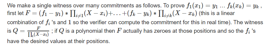
We make a single witness over many commitments as follows. To prove f_1(x_1) = y_1 … f_k(x_k) = y_k, first let F = (f_1 - y_1) * \prod_{i \ne 1} (X - x_i) + ... + (f_k - y_k) * \prod_{i \ne k} (X - x_k) (this is a linear combination of f_i's and 1 so the verifier can compute the commitment for this in real time). The witness is Q = \frac{F}{\prod_i (X - x_i)}; if Q is a polynomial then F actually has zeroes at those positions and so the f_i's have the desired values at their positions.

FRI-based commitments

We store the state in evaluations of a 2D polynomial F(x, y) with degree sqrt(N) in each variable, and we commit to evaluations of F on a 4*sqrt(N) by 4*sqrt(N) square.

We store any values we care about at positions (x, x**sqrt(N)) so they all have unique x coordinates. (Note that in many cases these positions will be outside the 4*sqrt(N) by 4*sqrt(N) square that we committed to evaluations on; this does not matter.)

To prove evaluations at a set of points x_1, ..., x_k we construct a degree-k polynomial path(x) whose evaluation at x_i is x_i**sqrt(N).

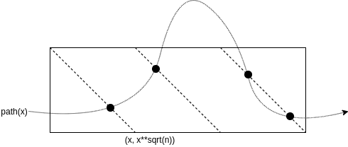
We then create a polynomial h(t) = F(t, path(t)), which contains all desired evaluations of (x_i, y_i) and has degree k * (1+sqrt(N)).

We choose a random 30 columns c_1 ... c_k within the evaluation domain, and for each column query a random 30 rows. We commit to h (with a FRI to prove that it actually is a polynomial), provide a multi-opening for z_i = h(c_i) and perform a FRI on a random linear combination on the quotients of the columns (R_i - z_i) / (X - path(c_i)) to verify that the claimed values of h(c_i) are correct and hence that h(t) actually equals F(t, path(t)).

The reason for using 2 dimensions is that this ensures that we do not have to do any computation over all of F; instead, we need only do the computation over the random 30 rows of F that we chose (that’s 30 * sqrt(N) work), plus h which has degree p * (sqrt(N) + 1), which is about p * sqrt(N) work to make a FRI for. This technique can be extended to higher than 2 dimensions to push the sqrt factor down to an even lower exponent.

Efficient writing

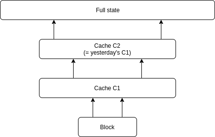
We get around the challenges associated with updating a single commitment containing the entire state by instead splitting the state into a series of commitments; you can think about it as being a “full state” with a series of “caches” in front of it. The full state is larger but is updated less frequently, whereas the caches are updated more frequently:

• The block itself, with a “read witness” (R_k(x), R_v(x)) and a “write witness” (W_k(x), W_v(x)) expressing the values to be written to the state. Note that we could set W_k = R_k and compute W_v at runtime.
• The first cache C1 = (C1_k(x), C1_v(x)) storing the last day of updates.
• The second cache C2 equal to the final C1 of the previous day.
• The full state S = (S_k(x), S_v(x)) containing values older than 1-2 days.

The approach that we will use to encode the state into S, C2 and C1 (each of which being represented by two polynomials, one storing keys and the other storing the corresponding values) is as follows. To read some key k from the state we will read C1, C2, S in that order. If C1_k(x) = k for some x then we read the corresponding value at C1_v(x) . Otherwise, if C2_k(x) = k for some x then we read the corresponding value at C2_v(x). Otherwise, if S_k(x) = k for some x then we read the corresponding value at S_v(x). And k is nowhere to be found in the evaluations of C1_k, C2_k or S, then the key is not part of the state so we return zero.

Intro to copy constraint arguments

Copy constraint arguments are a key ingredient of the witness update proofs we will use; see here for more details on how a copy constraint argument works. Briefly the idea is to pick a random r and generate an “accumulation” polynomial ACC(x) where ACC(0) = 1 and ACC(x+1) = ACC(x) * (r + P(x)). You can read the accumulator of the points in some range x....y-1 by opening reading ACC(y) / ACC(x). You can use these accumulator values to compare these evaluations to some other set of evaluations as a multi-set, without regard for permutation.

---

---

You can also prove equivalence of tuples of evaluations (ie. the multiset {(P_1(0), P_2(0)), (P_1(1), P_2(1)), ...}) by setting ACC(x+1) = ACC(x) * (r + P_1(x) + r2 * P_2(x)) for some random r and r2. Polynomial commitments can be used to efficiently prove these claims about ACC.

To prove subsets, we can do the same thing, except we also provide an indicator polynomial ind(x), prove that ind(x) equals 0 or 1 across the entire range, and set ACC(x+1) = ACC(x) * (ind(x) * (r + P(x)) + (1 - ind(x))) (ie. at each step, multiply by r + P(x) if the indicator is 1, otherwise leave the accumulator value alone).

In summary:

• we can prove the the evaluations of P(x) between a and b is a permutation of the evaluations of Q(x) between a and b (or some different c and d)
• we can prove that the evaluations of P(x) between a and b is a subset of a permutation of the evaluations of Q(x) between a and b (or some different c and d)
• we can prove that the evaluations of P(x) and Q(x) is a permutation of R(x) and S(x), where P -> Q and R -> S are the same permutation

In the next section, unless specified explicitly, we will be lazy and say "P is a permutation of Q" to mean "the evaluations of P between 0 and k are a permutation of the evaluations of Q between 0 and k for the appropriate k". Note that the next section assumes we also keep track of a “size” for each witness that determines which coordinates in any C_k we accept; out-of-range values of C_k(x) of course do not count.

Map merging argument

To update the caches we use a “map merging argument”. Given two maps A = (A_k(x), A_v(x)) and B = (B_k(x), B_v(x)) generate the merged map C = (C_k(x), C_v(x)) such that:

• the keys in C_k are sorted
• (B_k(i), B_v(i)) is in C for every 0 <= i < size(B)
• (A_k(i), A_v(i)) is in C for every 0 <= i < size(A) only if A_k(i) is not within the set of evaluations of B

We do this with a series of copy-constraint arguments. First, we generate two auxiliary polynomials U(x), I(x) representing the “union” and “intersection” of A_k and B_k respectively. Treating A_k, B_k, C_k, U, I as sets we first need to show:

• A_k ⊆ U
• B_k ⊆ U
• I ⊆ A_k
• I ⊆ B_k
• A_k + B_k = U + I

We pre-assume lack of duplication in A_k and B_k, meaning A_k(i) != A_j(j) for i != j within the range and the same for B_k (because that was verified already in the previous use of this algorithm). Because I is a subset of A_k andB_k we already know that I has no duplicate values either. We prove lack of duplication in U by using another copy constraint argument to prove equivalence between U and C_k, and prove that C_k is sorted and duplicate-free. We prove the A_k + B_k = U + I statement with a simple copy-constraint argument.

To prove that C_k is sorted and duplicate-free, we prove C_k(x+1) > C_k(x) across the range 0...size(C_k). We do this by generating polynomials D_1(x), ..., D_16(x) and prove C(x+1) - C(x) = 1 + D_1(x) + 2**16 * D_2(x) + 2**32 * D_3(x) + .... Essentially D_1(z), ..., D_16(z) store the differences in base 2**16. We then generate a polynomial E(x) which satisfies a copy-constraint across all of D_1, ..., D_16 along with f(x) = x, and satisfies the restriction that E(x+1) - E(x) = {0, 1} (a degree-2 constraint over E). We also check E(0) = 0 and E(size(C_k) * 16 + 65536) = 65535.

The constraints on E show that all values in E are sandwiched between 0 and 65535 (inclusive). The copy constraint to D_i proves that all values in D_i(x) are between 0 and 65535 (inclusive), proving that it is a correct base-16 representation, and thereby proving that C_k(x+1) - C_k(x) actually is a positive number.

Now we need to prove values. We add another polynomial U_v(x), and verify:

1. (U, U_v) at 0...size(B) equals (B_k, B_v) at 0...size(B)
2. (U, U_v) at size(B) ... size(A)+size(B) is a subset of (A_k, A_v) at 0...size(A)

The intention is that in U we put all the values that come from B first, and then the values that come from A later, and we use a same-permutation argument to make sure keys and values are copied correctly. We then verify that (C_k, C_v) is a permutation of (U, U_v).

Using the map merging argument

We use the map merging argument as follows. Suppose there are BLOCKS_PER_DAY blocks per day.

• if block.number % BLOCKS_PER_DAY != 0 we verify (C1_k, C1_v) = merge((W_k, W_v), (C1_old_k, C1_old_v)) (merging the block into C1)
• if block.number % BLOCKS_PER_DAY == 0 we verify (C1_k, C1_v) = (W_k, W_v) and (C2_k, C2_v) = (C1_old_k, C1_old_v) (that is, we “clear” C1 and move its contents into C2)

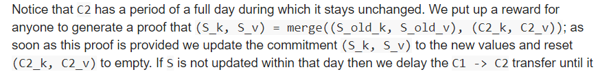
Notice that C2 has a period of a full day during which it stays unchanged. We put up a reward for anyone to generate a proof that (S_k, S_v) = merge((S_old_k, S_old_v), (C2_k, C2_v)); as soon as this proof is provided we update the commitment (S_k, S_v) to the new values and reset (C2_k, C2_v) to empty. If S is not updated within that day then we delay the C1 -> C2 transfer until it is updated; note that the protocol does depend on S being updated fast enough. If this cannot happen, then we can solve this by adding a hierarchy of more layers of caching.

Recovering from bad FRI

In the FRI case, note that there is a possibility that someone generates a FRI that’s invalid in some positions but not enough to prevent verification. This poses no immediate safety risk but could prevent the next updater from generating a witness.

We can solve this in one of several ways. First of all, someone who notices that some FRI was generated incorrectly could provide their own FRI. If it passes the same checks, it is added to the list of valid FRIs that the next update could be built off of. We could then use an interactive computation game to detect and penalize creators of bad FRI. Second, they could provide their own FRI along with a STARK proving that it’s valid, thereby slashing the creator of the invalid FRI immediately. Generating a STARK over FRI is very expensive, especially at the larger scales, but would be worth it, given the possibility of earning a large portion of the invalid proposer’s deposit as a reward.

---

And thus we have a mechanism for using polynomial commitments as an efficiently readable and efficiently writable witness to store the state. This lets us drastically reduce witness size, and also allows benefits such as giving us the ability to make data availability checks or proofs of custody on the state.

Future work

• Come up with a FRI proof that requires less than ~900 (more formally, less than square in the security parameter) queries
• It’s theoretically possible to update Kate commitments quickly if you pre-compute and store the Lagrange basis (L_i(x) = 1 at x = w^i and 0 at other roots of unity). Could this be extended to (i) quickly update all witnesses, and (ii) work for a key-value map and not a vector?

[bharathrao]

To prove non-membership of some keys one could try to construct a fancy proof that a key is not in S_k(1), ..., S_k(N) . Instead we simply sort the keys so that to prove non-membership it suffices to prove membership of two adjacent keys, one smaller than the target key and one larger.

This is insufficient. There also needs to be proof that the smaller key and larger key are in fact, adjacent.

[marcovasapollo]

But if the keys’ indexes are sorted during the writing phase, according to you, can this problem be bypassed?

[vbuterin]

It’s not a big deal; the witness would have to include the indices at which the keys are stored in any case, so that implicitly includes a proof that they are adjacent.

[dankrad]

@vbuterin

We make a single witness over many commitments as follows. To prove f1(x1)=y1f_1(x_1) = y_1 … fk(xk)=ykf_k(x_k) = y_k , first let F=(f1−y1)∗∏i≠1(X−xi)+…+(fk−yk)∗∏i≠k(X−xk)F = (f_1 - y_1) * \prod_{i \ne 1} (X - x_i) + … + (f_k - y_k) * \prod_{i \ne k} (X - x_k) (this is a linear combination of fif_i 's and 11 so the verifier can compute the commitment for this in real time). The witness is Q=F∏i(X−xi)Q = \frac{F}{\prod_i (X - x_i)} ; if QQ is a polynomial then FF actually has zeroes at those positions and so the fif_i 's have the desired values at their positions.

It is a linear combination but the factors are polynomials – doesn’t that mean that a full recompute of the commitments is necessary?

@vbuterin

(U, U_v) at size(B) ... size(A)+size(B) is a subset of (A_k, A_v) at 0...size(A)

I think you mean equals (A_k, A_v) here?

[vbuterin]

It is a linear combination but the factors are polynomials – doesn’t that mean that a full recompute of the commitments is necessary?

Yes. The goal is not to improve efficiency, the goal is to have a scheme that can hold more storage slots than the size of the trusted setup.

[Kama]

Does the different f_i represent the polynomail of the different cache(C1,C2)? So we only need to calculate once to verify if this point is included in the state.???

[Kama]

can I think this to be “proof of merge” replace “POW”?

[vbuterin]

Does the different f_i represent the polynomail of the different cache(C1,C2)? So we only need to calculate once to verify if this point is included in the state.???

You could use it for that. You could also use it to split the state across many polynomials to reduce the required trusted setup degree.

can I think this to be “proof of merge” replace “POW”?

Sure, you can call it “proof of merge” if you want Though it’s not a consensus algorithm so it doesn’t have anything to do with PoW or PoS.

[OlivierBBB]

Two questions on map merging. From your blog post on PLONK:

In PLONK, these polynomials depend on the circuit architecture alone (if one agrees on some wiring conventions). They are known to the verifier and the prover in advance, as are their (Kate) commitments.

In the map merging scheme you propose, it seems if one wants to convince oneself of the merging and ordering argument, one would have to compute a polynomial interpolating the one to one mapping

range( # of disctinct keys) —> range ( # of keys in A_k + # keys in B_k )
x |—> the index of the first occurrence of the x’th key (in ascending order) in A_k U B_k

Question 1 / looking for confirmation. The associated interpolating polynomial would have to be computed for every merge seemingly by anyone wanting to validate the supposed merge. If Kate commitments are involved, this would also involve a multiexponentiation.

EDIT. Ok, the problem I have below is really about how to prove both A_k \subset U and B_k \subset U. When producing the P and P’ that accumulate “the same points in the plane up to reordering the x coordinates when the y coordinates are equal” one is “linearly” going through the values of y : Y(1), Y(\omega), Y(\omega^2), … , Y(\omega^n), but that won’t be the case for U as there can be “gaps”. I don’t think there’s an actual problem: one should create U by including first the elements of A not in B, then the intersection of A and B, and then the elements of B not in A. Then the keys of A and the keys of B will both be consecutive in U, however those of B will start with an “offset”. Does this make sense, and is it a problem?

Question 2 / potential problem. The values from A_k one one wants to include won’t be consecutive: there will be “gaps”. For instance if A_k(1) is a key that isn’t already in B_k, A_k(2) isn’t, but A_k(3) is, we will want to include A_k(1) and A_k(3) but not A_k(2). Thus, it seems to me we aren’t sequentially including the keys, and so the condition p(x+1) = p(x) * (v + \sigma (x) + u A_k(x)) is meaningless for x = n + 2 (or p(\omega * x) = p(x) * (v + \sigma (x) + u A_k(x)) for x = g * \omega ^ 2). Is this a valid critique?

[vbuterin]

So we don’t actually need permutation polynomials here. In PLONK, we are trying to enforce that a set of wires is a specific permutation of another set of wires (or of itself). Here, we are just trying to enforce that the new commitment is any permutation of the old commitment plus the changes. The latter is actually easier to do than the former; in fact, the “specific permutation” argument is built out of the “any permutation” argument.

The keys are indeed not necessarily copied consecutively because there could be gaps.

The polynomial p for which you are applying p(x+1) = p(x) * .... is not the polynomial that we’re proving permutations of, it’s the “accumulator” polynomial that’s used to prove the permutation argument.