It’s widely recognized that CEX/DEX arbitrage trades create a large part of DEX volume, perhaps even the majority of that volume. The Loss Versus Rebalancing (LVR) model stands out as a key tool for quantifying and modeling this arbitrage volume from a theoretical perspective. However, the research focusing on LVR so far has mostly ignored transaction cost as a parameter in CEX/DEX arbitrage.
This post aims to extend the LVR model to blockchains such as Ethereum’s mainnet, where CEX/DEX arbitrage transactions are expected to have a significant fixed cost term. It conceptualizes LVR as a quantity that is distributed between three primary actors: (1) the LPs of the AMM, (2) the searcher-builder-proposer (SBP) as an aggregate entity, and (3) ETH holders, due to the block basefee that is burned by each transaction. Some implications are:
- As the block time is decreased, an increased share of the nominal LVR is spent on transaction fees.
- Liquidity provider (LP) losses from arbitrage trades do not have the same magnitude as the profits of the arbitrager (searcher-builder-proposer), and as such, are not accurately predicted by a model that approximates them with the square root of the block time.
- Changes in Ethereum’s block time (either increase or decrease) are expected to affect the profitability of AMM LPs, but in many situations, other factors are more important, including the transaction fees.
A more explanatory and less formal version of this post is available on Medium.
Background
According to (Millionis 2022, Millionis 2023) the expected instantaneous LVR is :
\overline{\mathrm{LVR}} \triangleq \lim _{T \rightarrow 0} \frac{\mathrm{E}\left[\mathrm{LVR}_T\right]}{T}=\frac{\sigma^2 P}{2} \times y^{* \prime}(P) .
This quantity depends only on the volatility, price, and marginal liquidity of the pool. By integrating the expected instantaneous LVR over time, we can obtain the expected LVR for a time period t. Once again, it is not dependent on external factors such as swap fees, block times, transaction costs, etc., and can serve as a nominal baseline metric for any further investigations in this area.
In (Millionis 2023) the authors push their LVR model further, and consider a situation when the AMM has a trading fee γ ≥ 0, and that arbitrageurs arrive to trade on the AMM at discrete times according to the arrivals of a Poisson process with rate λ > 0. They extend the asymptotic analysis of arbitrage profit in a fast block regime (\lambda \rightarrow \infty). They establish a key result that \overline{ARB} = Θ( \sqrt{λ^{-1}} ), where \overline{ARB} is the expected arbitrage profits over time. The authors do not explicitly discuss the case when block times are not Poisson distributed, however, intuitively, one can expect the approximation to remain reasonably accurate when the blocks are uniformly distributed. To formalize this idea: \overline{ARB} = Θ( \sqrt{BT} ), where BT is the average block time.
One key question is whether we see this formula play out in real-world data? A group of research papers generally confirm the \sqrt{BT} model:
- (McMenamin 2023) draws an analogy between the model and the time value of options, which “typically grows proportionally to the square root of time to expiration.”
- (Adams 2024) describe shorter block times as a reason for increased fee returns for liquidity providers, stressing the difference between Optimism and Arbitrum, in favor of later due to shorter blocks.
- (Fritsch 2024) empirically study the arbitrage profits predicted by the LVR model, and conclude that “our empirical findings come close to [the \sqrt{BT} model] for most pairs and block times larger than 1s”, and attempt to explain any deviations as a result of: (1) uniform block times (i.e. not Poisson-distributed), and (2) price action that does not match the Geometric Brownian motion (GBM) model. Their work is a step towards verifying the \sqrt{BT} model – however, it must be stressed that they measure arbitrage profits, not the LP losses.
In contrast:
- (Dahi 2023) investigate AMM on the XRP ledger and find only a tiny impact on the LPs: 0.35% in relative terms, if block time in simulations is reduced from 12 seconds to 4 seconds. This is much smaller than predicted by the \sqrt{BT} model.
- The Uniswap Foundation’s LP strategies series include simulation results that show a limited dependence on the block time, overshadowed by other factors.
How do we reconcile these differing results and bridge the gap between theory and practice?
The LVR model treats the arbitrage problem as a two-player, zero-sum game, where \overline{ARB} = - \overline{LP} (where the latter term refers to the expected LP profits). However, this assumption is not valid in the post EIP-1559 world, where transactions cannot be free. Each arbitrage trade not only divides profits among the searcher, builder, and proposer (“SBP” further in this article) but also burns some ETH, contingent on the blockspace demand at the time of the arbitrage. To borrow a term from physics, the basefee introduces a friction in the process. This friction eliminates a significant portion of potential trades, and reduces LP income.
Analyzing the single-trade LVR
Let’s look at the details of how LVR arises in real-world arbitrage trades. The difference between the DEX and CEX quoted prices (P_{DEX} and P_{CEX}) triggers the arbitrage trade. However, the trade is not going to happen if:
- The CEX price is in the non-arbitrage region created by AMM’s swap fees.
- The CEX price is in the friction region, created by the chain’s basefees and other factors (CEX fees, other operational costs for arbitrager, risk aversion, etc.).
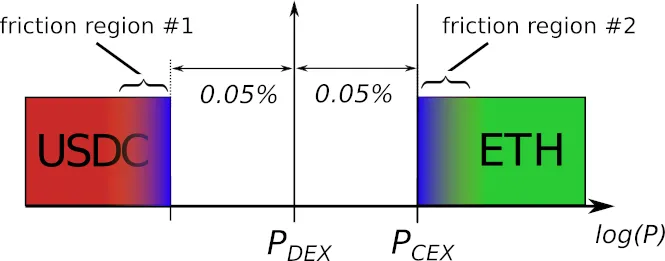
Figure 1: Non-arbitrage and friction regions of an AMM pool with 0.05% swap fee.
Moreover, the nominal single-trade LVR is “distributed” between three entities:
- Liquidity providers.
- The searcher, block builder, and block proposer (SBP) as a collective entity.
- Holders of ETH, due to the ETH burned in the transaction.
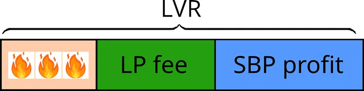
Figure 2: The nominal LVR is distributed between three entities: ETH holders (due to the burned basefees), LPs, and the searcher/builder/proposer as a collective entity.
LPs receive the swap fee, while the SBP collects the arbitrage profits, which are subsequently divided among these three actors. It’s no surprise that integrated searchers-builders dominate the arbitrage market (Heimbach 2024), as for them it is simpler to divide up the profits. ETH holders do not directly receive compensation, but burning the basefee creates a deflationary pressure on ETH as an asset.
By comparing the nominal single-trade LVR with the LP fees from that trade, we can assess the fairness of the trade to the LP. In a scenario where price evolution is smooth without any jumps, the LP fee nearly recoups the LVR, and the LP loss is minimal. However, if the DEX-to-CEX price difference fluctuates due to block time granularity or actual price discontinuities on the CEX, the LP fee becomes smaller than the LVR, resulting in some loss for the LP against the theoretical rebalancing strategy. One example is shown in the figure below:

Figure 3: Distribution of the LVR between the three actors. Relative scale. The LVR created by 0.1 % price changes has a much more equitable distribution than the LVR created by 1.0% price change at once.
Computing the nominal LVR
Let’s assume that we are a given sequence of CEX prices at BT intervals and a constant product AMM (i.e. AMM that follows the equation xy=k). In order to compute the empirical approximation of the nominal LVR defined as above, we can use the following algorithm:
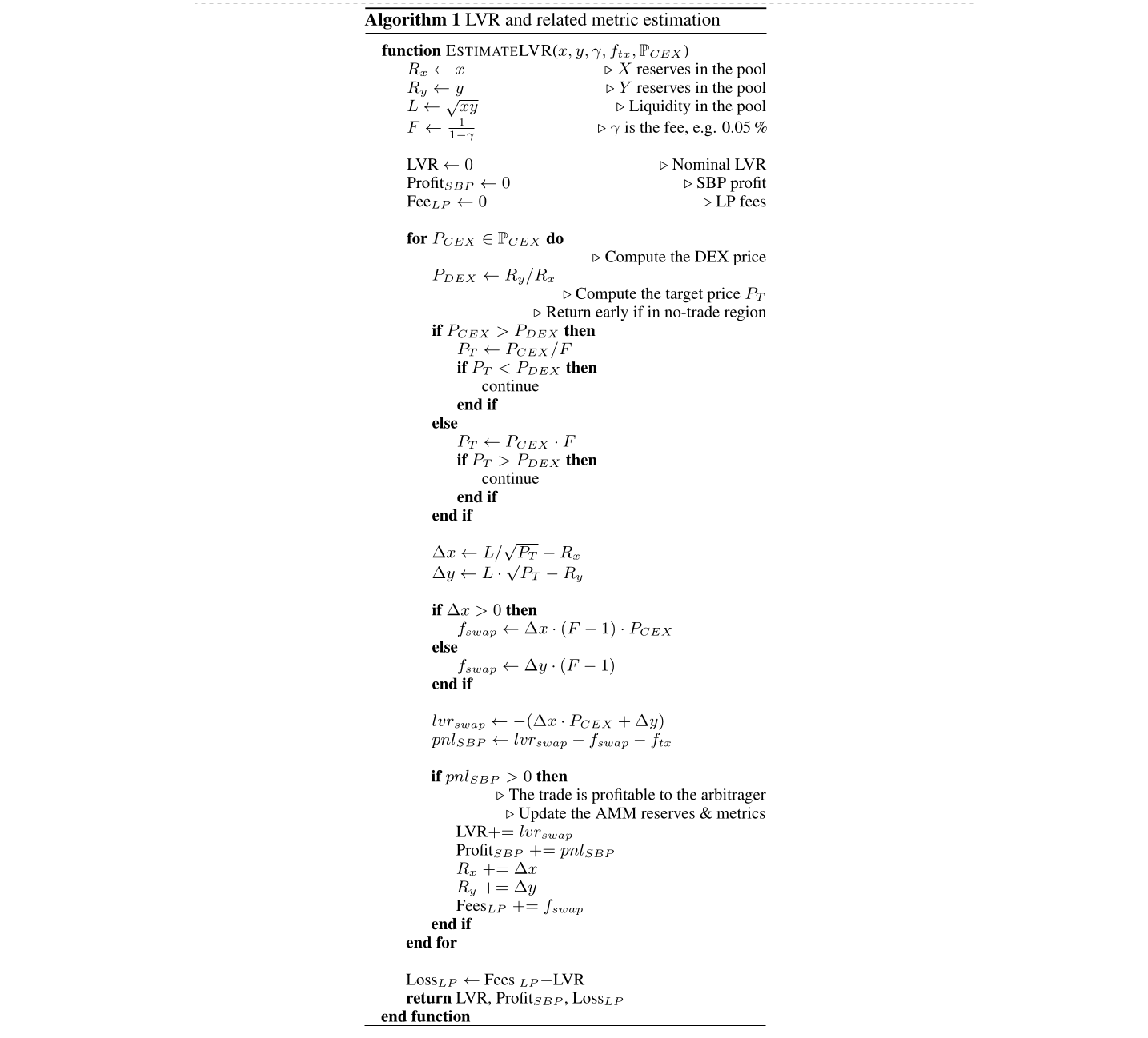
The results of the algorithm have been verified to match both the nominal LVR and the arbitrage trade probability as defined in (Millionis 2023) – see “Replicating the theoretical results” section in the Medium post.
Simulation studies
Let’s model the in-range liquidity of the Uniswap v3 ETH/USDC 0.05% pool. As of April 2024, it has approximately $1 billion worth of virtual assets, corresponding to approximately $150 millions of real assets. As a result, the liquidity concentration factor is between 6 and 7. It’s essential to have deep liquidity if we want arbitrage swaps to happen even on relatively small price changes.
The graphs below show the DEX performance metrics using random GBM simulations. The simulations assume 50% yearly volatility, which corresponds to approximately 2.6% daily volatility and 0.03% per-block volatility for 12-second blocks. This is the approximate volatility of ETH in the recent years.
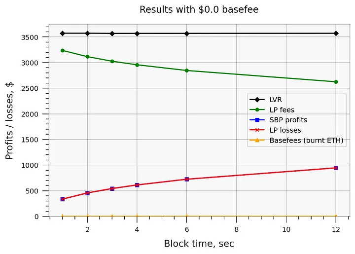
Figure 4: Simulated DEX metrics with zero basefee.
Due to a coincidence, the LVR turns out to be approximately $1 per second or $3600 per hour. The LP losses in turn are in the range from $350 to $900 per hour ($3 to $8 million per year). To be clear, this theoretical model does not include any LP fees coming from noise / uninformed traders, which are expected to produce zero LVR, and consequently compensate for the LP losses from the arbitrage trades.
The results show that when the basefee is zero, the LP losses indeed can be more-or-less accurately modeled by the function \sqrt{BT}. However, after introducing EIP-1559 basefees to the model, this isn’t true anymore.
The subsequent two graphs show what happens with when each transaction is assumed to cost a fixed amount of $. A simple Uniswap v3 swap might consume around 150’000 gas, which corresponds to $10 cost per swap in USD terms – assuming the reasonable 22 gwei basefee cost and $3000 ETH/USDC price. In times of high usage or high volatility, the cost of a transaction can easily increase several times.
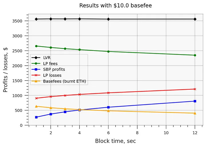
Figure 5: Simulated DEX metrics with $10 per swap spent on the basefee.
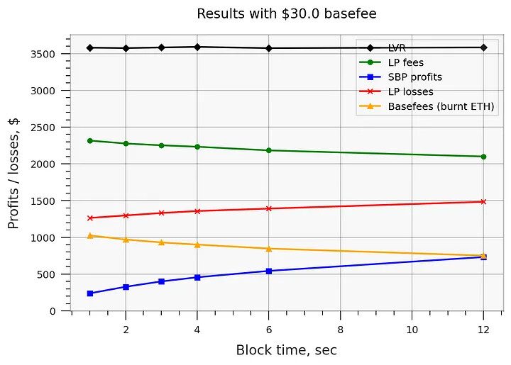
Figure 6: Simulated DEX metrics with $30 per swap spent on the basefee.
For a summary of the LP losses, see the figure below. Even adding a constant offset from the x axis to the \sqrt{BT}. model does not lead to a good fit (the brown line). More frequent transactions also burn more ETH, thus canceling out most of the positive impact on the LP fees.
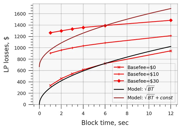
Figure 7: The \sqrt{BT} model shows a good-but-not-perfect fit if the basefee is zero, but much worse otherwise.
Simulations with longer block times
Following Table 1 in (Millionis 2023), I also include results with 120 second and 600 second blocktimes.
Uniformly distributed blocks, $10 swap basefees:
swap fee:                          1bp   5bp  10bp  30bp 100bp
block time   600 sec, arb prob %: 92.7  85.2  76.4  50.5  21.7
block time   120 sec, arb prob %: 83.7  68.4  53.5  27.4   9.9
block time    12 sec, arb prob %: 53.1  29.9  19.1   7.7   2.0
block time     2 sec, arb prob %: 20.8   9.4   5.5   1.8   0.1
swap fee:                          1bp   5bp  10bp  30bp 100bp
block time   600 sec, LP loss  %: 96.3  83.5  71.3  44.8  19.6
block time   120 sec, LP loss  %: 92.1  69.1  52.5  26.9  10.0
block time    12 sec, LP loss  %: 80.0  44.2  28.3  11.6   3.8
block time     2 sec, LP loss  %: 69.6  31.3  18.6   7.1   2.2
Uniformly distributed blocks, $30 swap basefees:
swap fee:                          1bp   5bp  10bp  30bp 100bp
block time   600 sec, arb prob %: 88.8  81.5  72.8  48.1  20.8
block time   120 sec, arb prob %: 75.4  61.0  47.8  24.5   8.8
block time    12 sec, arb prob %: 36.2  21.3  14.0   5.8   1.5
block time     2 sec, arb prob %: 10.7   5.5   3.3   1.1   0.1
swap fee:                          1bp   5bp  10bp  30bp 100bp
block time   600 sec, LP loss  %: 96.3  83.6  71.4  45.0  19.8
block time   120 sec, LP loss  %: 92.3  69.8  53.3  27.6  10.3
block time    12 sec, LP loss  %: 82.5  48.5  32.0  13.5   4.5
block time     2 sec, LP loss  %: 76.5  39.5  24.6   9.8   3.2
The results show that:
- The approximation from (Millionis 2023) that arbitrage probability is approximately equal to LP loss does not hold, in general.
- In most cases, the swap fee is a more dominant factor for the LPs than either the block time or basefee.
- Increasing the block time does increase LP losses, but by a much smaller factor than predicted by the \sqrt{BT} model, especially in pools with low swap fees (1 bps to 10 bps).
Discussion
Generalizing the results
-
Generalizing to other pools. The simulation results above are specific to the USDC/ETH 0.05% pool, which is typically the most liquid volatile pool on Uniswap v3. (There are stable pools with deeper liquidity). For pools with lower liquidity, the importance of the friction created by the basefee would be increased. For instance, let’s say that the ETH/USDT 0.05% pool has 1/3 of the liquidity. Then the results from $10 basefee on that pool would match those of the USDC/ETH pools with $30 basefee. For pools with higher liquidity (such as USDC/USDT) the friction would be decreased, proportional to the rise in liquidity.
-
Generalizing to other chains. The model assumes that shorter blocks simply divide the available blockspace differently, rather than add more blockspace. The simulation results would not generalize if the block time decrease was accompanied with a proportional decrease in basefees.
Implications for blockchain design
The results clearly show that LP losses are not accurately predicted by the \sqrt{BT} model, unless the basefee is close to zero. While it’s true that shorter blocks benefit LPs, the effect is limited and frequently less significant than other factors (basefee, liquidity depth, swap fee %, and potentially others). More compelling arguments for fast block times may come from other perspectives, like the perspective of traders, or that of block builders, but these are out of the scope for this article.
Potentially, we can view the optimal block time choice problem from two viewpoints:
- From L1 perspective, reducing the basefee could provide a quicker win, compared with changing the block time. However, keeping the design decentralized and credibly-neutral is arguably a higher priority.
- From L2 / appchain perspective, especially for chains that focus on DeFi or on trading in particular, it makes sense to excessively optimize for LP profits, including block time and basefee reduction.
-
- The \sqrt{BT} model implies that decreasing block times is especially important if the block time is already close to zero, since the \sqrt{~} function rapidly grows in the near-zero region.
-
- L2 fees may already be low enough to minimize the friction caused by the basefee to negligible levels. If this isn’t the case, then paradoxically, exempting CEX/DEX arbitrage swaps from the EIP-1559 basefee would benefit DEX users (both LPs and retail traders).
Shorter blocks = less MEV?
To be clear, this article makes no claims about MEV in general, just about CEX/DEX arbitrage in particular. Regarding the latter, clearly, there’s a connection between CEX/DEX arbitrage, transaction fees, and block times. However, it is perhaps confusing because this connection goes both ways:
- Shorter blocks increase the number of arbitrage transactions and the proportion of gas that they consume.
- On the other hand, shorter blocks decrease the expected value of LP losses.
The same conflicting results apply to changes in basefees. As a result, there’s potential for a confusion, because MEV is increased in one sense, and decreased in another sense.
Conclusion
This work extends the existing LVR and LVR-with-fees models by adding another component: transaction cost. To summarize the main results:
- CEX/DEX arbitrage transactions are not frictionless due to the EIP-1559 basefee and other factors.
- As a result, the nominal LVR in real-world AMMs is divided among three entities: LPs, ETH stakers, and the SBP as a collective entity.
- More gradual price changes result in more equitable LVR distribution among these three entities.
- On chains with significant transaction costs, LP losses under the LVR assumptions are not accurately predicted by the \sqrt{BT} model.
- The LP losses are determined by several factors, including basefees, swap fees, and block times, the relative importance of which varies.
Source code of the simulations is available here.