Thanks to Nethermind, @tkstanczak, @swapnilraj , @dapplion, Martin Koppelmann and @DrewVanderWerff for discussion, feedback and review.
This is the first instalment in a series of posts where I will outline a methodology for understanding and pricing gas derivatives. The following approach for pricing will be valuable for gas hedging and can also be applied to develop a subscription model for Ethereum.

There Will Be Blood” (2007) - are we going to be unwitting extras in the ‘digital oil’ sequel?
TLDR: I show how a two-factor model can be used to price base fee options, of both European and American type. A developed gas derivatives market would be highly beneficial for participants looking to hedge against volatile operational expenses on gas or for those aiming to speculate on future gas fee trends.
Why Price Base Fee Derivatives?
Gas expenditure is a substantial portion of operational costs within blockchain ecosystems. Whether it involves L2 sequencers committing transactions to L1, the running of a DeFi protocols keeper, interacting with oracle contracts, rebalancing liquidity on platforms like Uniswap, verifying proofs, or conducting arbitrage, gas fees are an unpredictable expense. This inherent volatility poses challenges for financial planning and budgeting in blockchain operations. Gas hedging, analogous to its counterpart in traditional financial markets, provides a mechanism to manage and mitigate this uncertainty.
By purchasing gas derivatives, stakeholders can secure current gas fee levels for future transactions, effectively insuring against unforeseen spikes in gas prices. Additionally, with a strike price of zero on a call option, one can fully prepay for gas, paving the way for a ‘gas subscription’ model on Ethereum—assuming a delivery mechanism is established. This research could be particularly useful for pre-confirmations, where blockspace is purchased in advance.
The following post breaks down the importance of understanding base fees, examining their volatility, and proposing a detailed model for pricing base fee derivatives. The first section delves into the calculation of base fees, while the second outlines their structure. In the third section, a model incorporating both deterministic and stochastic components is detailed to simulate base fees using a Monte Carlo process. The fourth and final section explains how to use these Monte Carlo generated paths to price base fee options, including both European and American types. Use cases of this research include participants that want to examine the fair value of a base fee option, a task helpful for those interacting with derivative protocols like Oiler’s Pitch lake [1].
This post is the first in a series on the topic, aimed at sparking interest among both Ethereum researchers and traders. My goal is to engage quants in the conversation around Ethereum infrastructure.
Understanding Base Fees
Before pricing base fees, we should understand its constituent parts. EIP-1559, implemented in the London hard fork of Ethereum in August 2021, introduced a significant overhaul to the transaction fee mechanism on the Ethereum network. The proposal aimed to improve the predictability and efficiency of transaction fees, addressing several issues inherent in the previous auction-based system. Under EIP-1559, each block has a base fee, which is dynamically adjusted according to network congestion. When demand for block space increases, the base fee rises, and when demand decreases, the base fee falls. This mechanism helps to stabilize transaction fees and makes them more predictable for users.
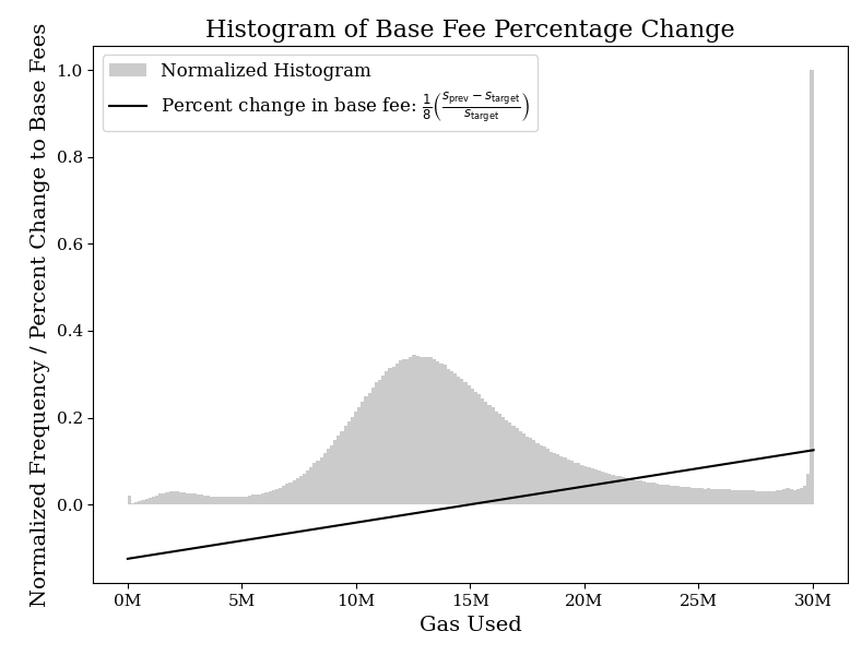
The specific adjustment rule proposed in the EIP-1559 spec computes the base fee BF_{\text{cur}} for the current block from the base fee BF_{\text{pred}} and size s_{\text{pred}} of the predecessor block using the following formula, where s_{\text{target}} denotes the target block size:
In short, the next base fee is adjusted by a percentage that equals one-eighth of the difference to the target percentage - meaning base fees are within the bounds of 12.5% higher or lower than the previous block. As is visible below when comparing gas usage, full blocks of 30M are most frequent, with gas usage of just below 13M second most frequent.
Those Are Some Large Percentage Changes… Why Are Base Fees So Volatile?
Several factors contribute to the high volatility of base fees, with the non-storability of base fees and the limited block-space supply being the most significant. Since block-space has a strict limit to 30M gas, which cannot be stored or transferred over time, supply in each time period is fixed, while demand can fluctuate based on usage needs. Base fees for transactions is thus demand inelastic. Consequently, during periods of low demand, the base fee remains relatively stable. However, during peak times, the relative insensitivity of demand to price changes can lead to significant volatility in short-term base fee prices—‘Jumps’. This situation is similar to the electricity market, where demand remains high regardless of price, causing extreme price volatility during peak usage. In the blockchain context, the necessity of paying the base fee to conduct transactions ensures somewhat steady demand, even as prices fluctuate dramatically.
Additionally, since base fees are influenced by the previous base fee, a block with high demand for blockspace—such as one resulting from the deployment of a large simultaneous smart-contract architecture—will primarily impact users in the following block. Users pay for blockspace based on the previous blocks usage, not the current one. Consequently, in the short term, a deployer will not always experience the negative externalities of increasing gas fees for near-future blockchain users. This creates a scenario where users are indifferent to increasing base fees by the cap of 12.5%. Current discussions, as well researched by SMG [2], suggest to minimise this externality, and subsequent short-term volatility by modifying the denominator to a higher value. The change would reduce sensitivity to randomness in gas usage and better align the process with underlying trends, improving stability and predictability.
Characteristics of Base Fees
Base fees can be simulated through understanding the structure of gas usage, before feeding the resulting parameters into the BF_{\text{cur}} equation to find the base fees, or observing base fees themself. The model I propose focuses on the latter, as a result of my focus being on hourly averaged base fees for use in 1 day plus dated options, and a focus on gas usage would also mean accounting for variable gas limits. The model I am proposing is very flexible, and allow us to simultaneously include trends, seasonality, mean reversion, volatility and jumps.
Overarching Trend
Unlike electricity, wherein supply can vary, base fees relate directly to the demand side usage of a product, a blockchain. When a new EIP is passed as to change the structure of base fees, or if gas usage dramatically decreases. Unlike electricity, trends in gas usage are far shorter and dissimilar to one another, trends should thus be likened to regimes. For example, one regime may be a simple horizontal linear trend in periods of stable usage, where another is an exponential trend downwards as a result of blobs being recently introduced.
Seasonality
Base Fee demand is heavily influenced by varying usage of economic and business activities of agents on the underlying blockchain. Different kinds of seasonality appear in the data; intra-daily and weekly. As it is usual in this type of research, I assume that seasonality is generated by deterministic factors and since I use the average hourly prices.
Mean-reversion
In the short term, during periods of high demand, base fees spike, discouraging excessive gas usage, which in turn reduces congestion and drives fees back down. Conversely, during low demand periods, lower fees encourage more transactions, increasing congestion and pushing fees back up. This cyclical nature of congestion creates a mean-reverting behaviour in base fees. Essentially, despite short-term fluctuations, base fees tend to stabilize around an average level, influenced by the balance of demand and network capacity.
Jumps and volatility
By simple eye inspection of base fees over time, there is clear existence of important jumps in the behaviour of base fees, as a result of sequential filling of blocks. One of the characteristics of evolution of these jumps is that the base fees do not stay in the new level, to which it jumps, but revert to the previous level rapidly. Such a behaviour can be captured by introducing a jump-diffusion component to a simulation model.
Pricing Base Fees
How should one price option premiums? Determining the appropriate pricing model for gas fees involves understanding their nature and selecting an appropriate financial framework. Gas fees could be treated as equities, interest rates, or commodities, each with distinct modelling approaches. Popular analytical models like the Black-Scholes closed-form model, often used for equities, offer theoretical insights into price movements and volatility - but in the case of base fees, the underlying assumption of normality in returns would be too naive, and the mean reversion and seasonality present in base fees wouldn’t be accounted for. Alternatively, numerical methods such as finite difference and Monte Carlo simulations would provide far more flexible and robust techniques for capturing the stochastic and path dependent nature of base fees. I therefore opt for the Monte Carlo simulation approach.
Model Specification and Estimation
Exponential Trend Examination
I first assess the presence of an exponential trend by computing the weekly statistics of the mean and standard deviation. If the spot price series exhibits an exponential trend, then the means and standard deviations, computed over time periods, should be correlated with a statistically significant slope.

Demonstrated by a p-value close to zero (4.43e-18), an exponential trend is evident in the data. When base fees are high, base fees are volatile. Consequently, to simplify modelling and work with linear trends, I from hereon out use the logarithm of the base fee.
Deterministic Model Specification
We have seen in the previous section that a reasonable model for base fee prices should allow for the existence of deterministic seasonality, the possibility of mean-reversion, seasonality jumps, and volatility (randomness). Therefore, I propose a model that simultaneously incorporates all these factors in a flexible way.
The combined long-term model can be written as the composite of a deterministic component f(t) and a stochastic component X_t:
Estimation of Deterministic Component f(t)
The deterministic component f(t) is given by the sum of piecewise regime-based quadratic polynomial trends and sinusoidal functions corresponding to different harmonics and periods:
Where:
- \log BF_t is the logarithm of the base fees per gasat time (t).
- t is the time in hours since the start of the sample.
- \beta_1 and \beta_2 are the coefficients for the fundamental daily seasonal components (1 day period).
- \beta_3 and \beta_4 are the coefficients for the first harmonic daily seasonal components (1 day period).
- \beta_5 and \beta_6 are the coefficients for the second harmonic daily seasonal components (1 day period).
- \beta_7 and \beta_8 are the coefficients for the fundamental weekly seasonal components (7 day period).
- \beta_9 and \beta_{10} are the coefficients for the first harmonic weekly seasonal components (7 day period).
- \beta_{11} and \beta_{12} are the coefficients for the second harmonic weekly seasonal components (7 day period).
- \mathbb{I}_{\{t \in R_i\}} is an indicator function that equals 1 if t is within regime R_i and 0 otherwise.
- \gamma_{i,0}, \gamma_{i,1}, and \gamma_{i,2} are the coefficients for the piecewise polynomial trend within regime R_i.
- \xi_t is the error term.
For each regime R_i, I fit a quadratic model of the form:
To discover the boundaries of each regime, I utilise binary segmentation for detection of change points within the time series. This technique employs a piecewise model, identifying changes based on the L2 norm (Euclidean distance). Initially, the algorithm treats the entire time series as a single segment, searching for a point that maximises the cost function by minimising the residual sum of squares. When a significant change point is identified, the segment is split, and the algorithm recursively continues this process until no further significant change points are found.
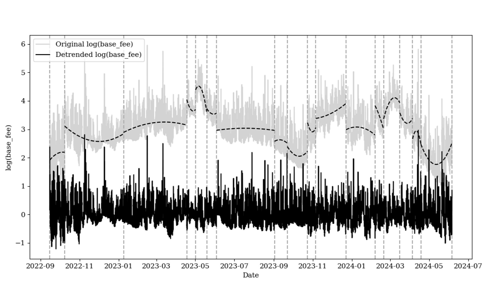
In our dataset of roughly two years, and discovered partially heuristically, I identify 16 change points, 17 regimes, with an initial regime immediately after EIP-1559’s release. This finding indicates that the underlying trend in base fees shifts approximately every half to two months. Such shifts are likely influenced by market events such as changes in market sentiment, or other critical factors, all of which could warrant their own focused research to fully understand their cause. I then discover the parameters \gamma_{i,0}, \gamma_{i,1}, \gamma_{i,2} for each regime R_i, using the least squares method. This involves minimising the sum of the squared differences between the observed values BF_t and the predicted values z_i(t) within each regime R_i:
To solve this minimisation problem, I set up the following normal equations by taking partial derivatives with respect to each parameter and setting them to zero:
Solving these equations yields the least squares estimates for \hat{\gamma}_{i,0}, \hat{\gamma}_{i,1}, \hat{\gamma}_{i,2} for each regime R_i. The below figure displays the resulting regimes and trend curves. The regression analysis has a low R^2 for the majority of regimes, indicating that the trends are well-fitted to the data. Notably, the current regime, characterised by the implementation of EIP-4844, differs markedly from the previous two regimes, as base fees dramatically decrease immediately after the fork, and are recovering upwards, likely due to the recent bull market activity. I eagerly ask for a discussion with respect to the underlying reasons for each trend.
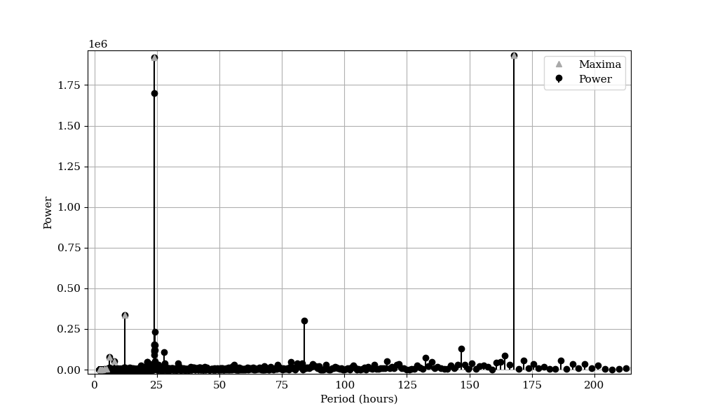
To calibrate the seasonality components, I first analyse the seasonality present within the data. To do so, I performed a spectral analysis using the Fast Fourier Transform (FFT). The FFT decomposes the time-domain signal into its constituent frequencies, allowing us to compute the power spectrum, which represents the signal’s power distribution across different frequencies. I focused on the positive half of the spectrum and converted frequencies to periods in hours. Significant periodic components were identified by locating peaks in the power spectrum. The identified cycles, with the most prominent displaying daily (24 hours) and weekly (168 hours) seasonality, reinforcing the sinusoidal functions specified above. I visualise the results below to highlight the dominant seasonal patterns in the data.
In estimating the \beta parameters, I also use a least squares optimisation method. Given the observed log base fees BF and the seasonality matrix C, the objective is to estimate the seasonality parameters \beta that minimise the sum of squared residuals. This is formulated as:
where:
- log(BF)_{detrended} is the vector of de-trended log base fees,
- C is the matrix containing the seasonality functions (sine, cosine),
- \beta is the vector of seasonality parameters to be estimated.
The expanded form of the objective function is:
where log(BF_i)_{detrended} is the i -th observed log base fee and C_i is the i-th row of the seasonality matrix. To find the least squares solution, I set the gradient of the objective function with respect to \beta to zero, yielding the normal equations:
Simplifying, I obtain:
Solving the normal equations for \beta provides the least squares estimates:
where (C^T C)^{-1} C^T is the Moore-Penrose pseudoinverse of C. The de-seasonalized and de-trended log prices are then calculated by subtracting the combined seasonality components from the observed log prices, as is shown in the figure below.
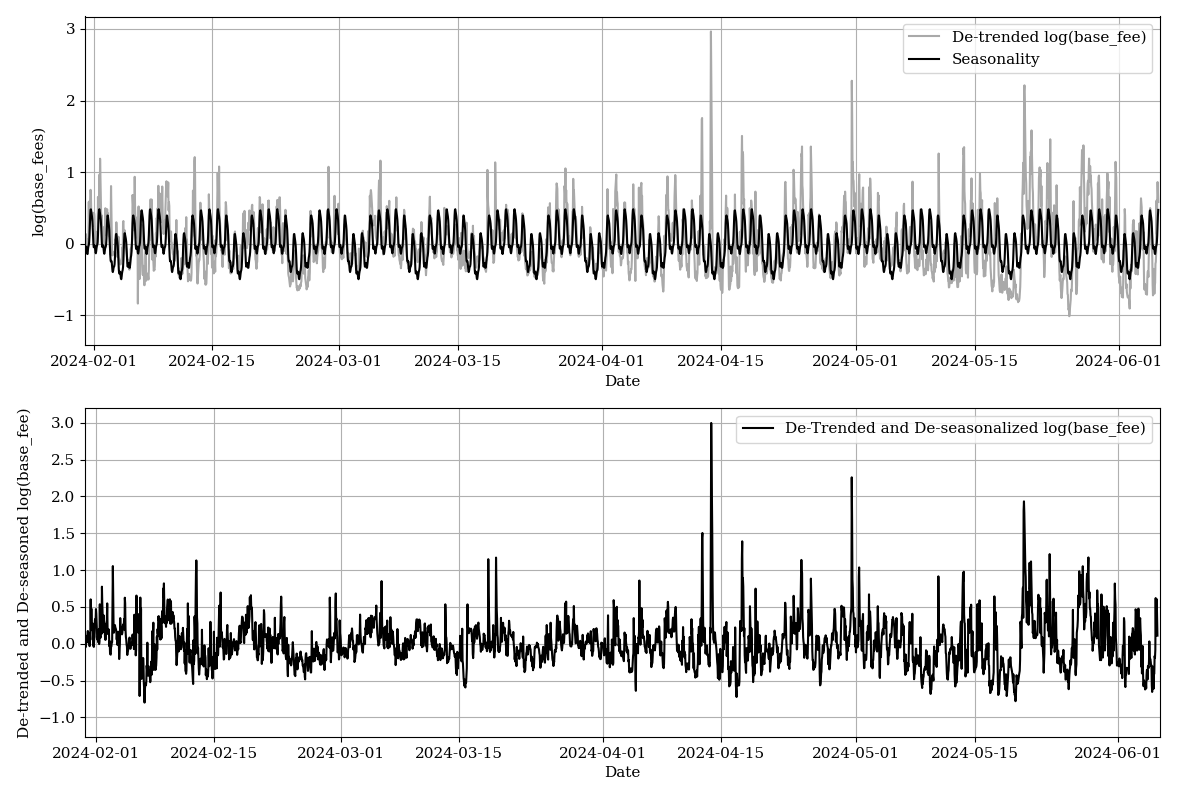
Visibly, base fees in the Ethereum network fluctuate due to weekly and daily patterns of usage. During the week, gas usage is typically higher as business activities, market trading, and development deployments peaks. This weekly seasonality contrasts with daily patterns where peak periods of gas usage occur in the morning and evening as global participants, including Europe and North America, overlap in activity.
Despite removing trend and overarching seasonality, I observe that autocorrelative structure is still present in our time series. To address this, I explore the autocorrelation function (ACF) and the partial autocorrelation function (PACF) of the data. The ACF helps identify the correlation between observations at different lags of base fees, providing insights into the persistence of shocks over time. The PACF isolates the direct effect of a lagged observation by controlling for the contributions of intermediate lags, aiding in the identification of the order of the autoregressive (AR) terms in an ARIMA model. By observing the graph below, we observe 34 autocorrelated lags, and 5 partially autocorrelated lags.
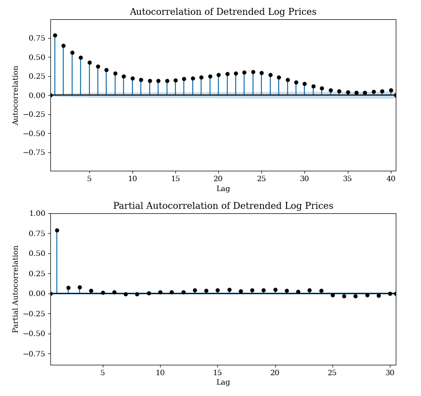
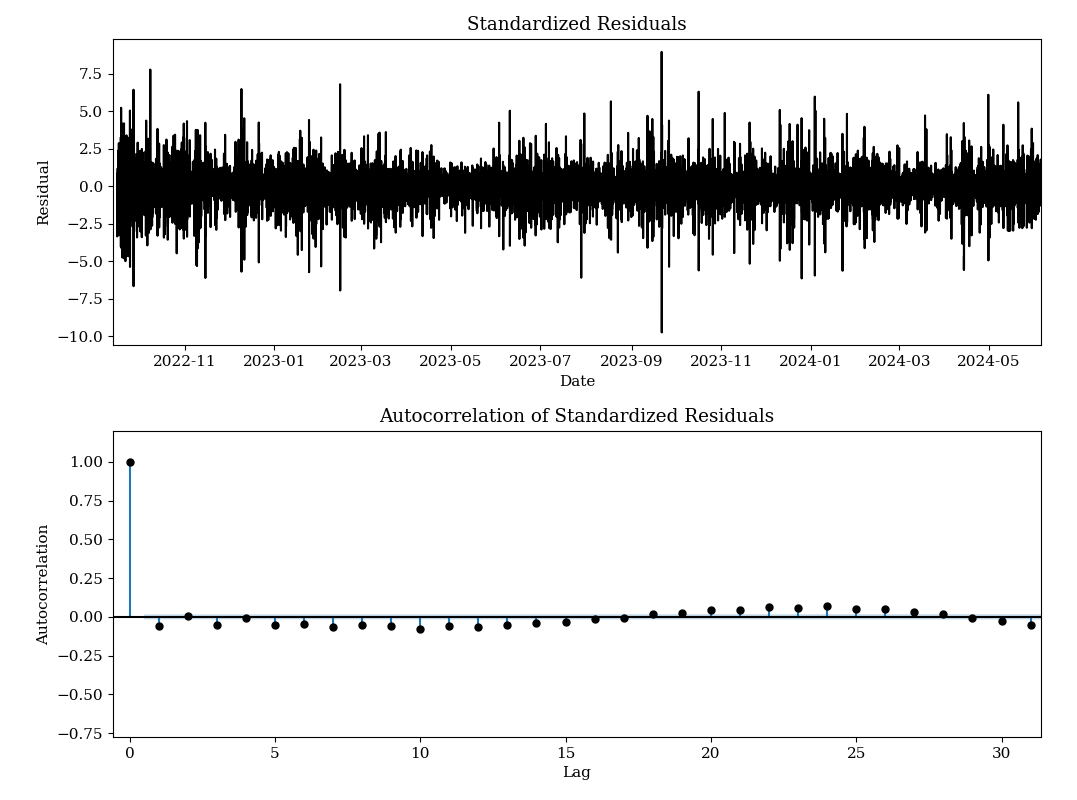
To address these lags, I fit an ARIMA(34, 5, 5) model to the de-seasonalized and de-trended data. This model captures the autoregressive and moving average components along with differencing. By fitting this model, we obtain the residuals, which represent the underlying structure of the noise after accounting for these components. Upon examining the residuals, we find that the distribution of the noise is sharply centered around zero with fat tails. The transition between the central peak and the tails appears to follow an exponential pattern. Consequently, we fit a Laplace distribution to the residuals and compare the observed values against the expected values, where the Laplace distribution is defined as:
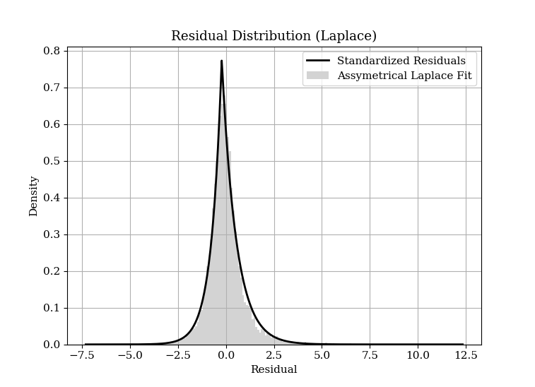
- \mu is the location parameter (mean),
- b > 0 is the scale parameter,
- \kappa > 0 controls the asymmetry of the distribution. a Kappa equal to 1 produces a symmetrical Laplace distribution.
A Laplace distribution is significant because it characterises the distribution as having exponential decay on both sides of the peak. In the context of Ethereum base fees, changes often occur as a percentage of the previous base fee rather than by fixed amounts. This implies that large deviations from the mean are more probable than would be expected under a normal distribution, leading to the characteristic heavy tails of the Laplace distribution. The sharp central peak of the Laplace distribution indicates a high probability of small changes around the long term mean. The fat tails, on the other hand, reflect the occasional large percentage changes, driven by significant network, a series of full block events or structural shifts in demand for block space. One would expect a higher denominator parameter (reducing sensitivity of base fees to gas usage) to create a ‘tighter’ distribution with a lower standard deviation.
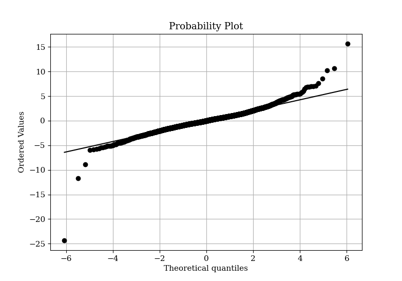
I plot the theoretical quantiles of the Laplace distribution against the observed residual quantiles in a QQ plot. The plot revealed that a few outlier observations exhibited fatter tails than predicted by the Laplace distribution, indicating that the residuals have more extreme values than our model accounts for. Nevertheless, the majority of the data points followed the expected distribution, suggesting that the Laplace distribution still provides a reasonable fit for the central portion of the residuals.
Stochastic Component Specification
Cox, Ingersoll & Ross Poisson Asymmetrical Laplace calibrated model
Removing the trend and observing the noise, the stochastic component X_t is modelled as an Ornstein-Uhlenbeck process (mean-reverting) with jumps, incorporating a Laplace distribution for both the noise term and the jump size
where:
- α is the drift parameter,
- κ is the rate of mean reversion,
- σ is the volatility,
- L_t is a noise term following a Laplace distribution,
- J(μ_J , σ_J ) is the jump size, following a Laplace distribution with mean μ_J and scale parameter σ_J ,
- Π(λ) is a Poisson process with jump intensity λ.
The transition probabilities for base fee equilibrium prices follow a Poisson-Laplace process. This can be expressed as:
where:
- ∆t is the time increment,
- a is the drift term,
- φ is the autoregressive coefficient,
- b is the scale parameter of the Laplace distribution.
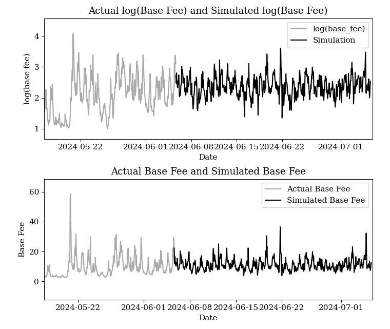
The parameters Q = {α, κ, σ, a, b, μ_J , σ_J , λ} can first be estimated by Maximum Likelihood (ML). This approach ensures that the parameters Q are optimised to best fit the observed data under the specified model. The results of the simulation, displayed below, demonstrate the simulated log base fees for the next month. Notably, considering the most recent regime of exponential increase, I adopt a neutral market approach by assuming a linear (horizontal) trend. For pricing derivative products, consideration of what the future trend will be should be taken into account. After retrieving calibrated parameters, a range of future hourly dates is produced, before trend and seasonality is added back in, and the exponential is taken to revert the log.
ARIMA Monte Carlo Method
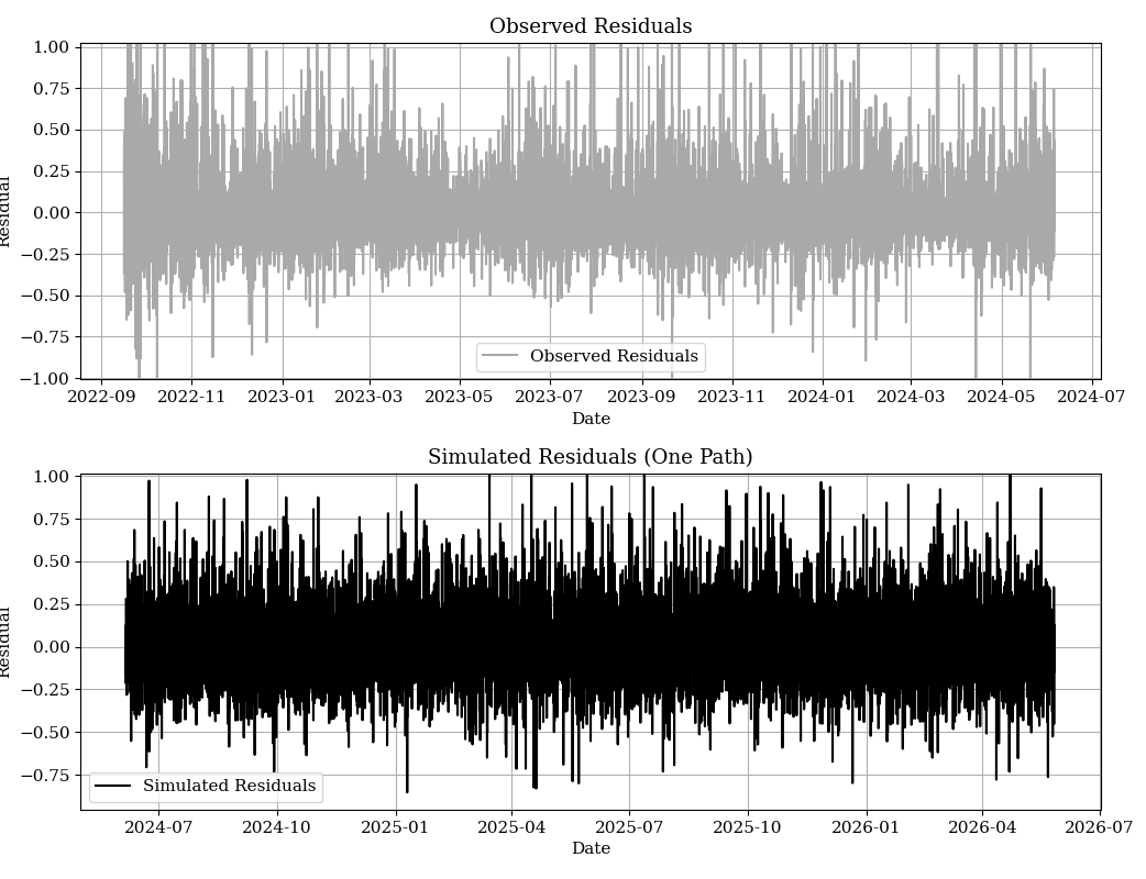
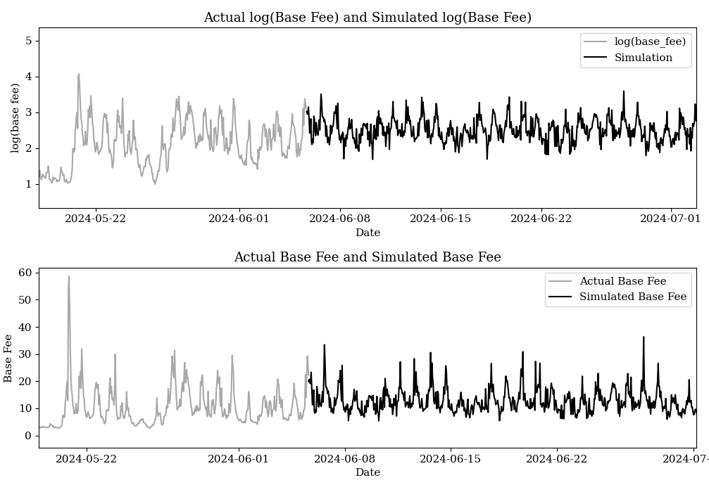
An alternative method, which requires less computation simulates a monte-carlo process by modelling standardised residuals directly from a Laplace distribution, augmenting these standardised residuals back de-normalising them, before generating future paths as the composite of both this noise and ARIMA forecasts. A simulated residual path is shown below, producing the resulting simulation.
Pricing with these simulated values
For the purpose of hedging, pricing a European call or put option based on the simulated paths can be expressed as follows. Let BF_T^i represent base fees per gas at maturity T for the i-th simulated path, where i = 1, 2, \ldots, N, and denote the strike price by K. The payoff for the European call option at maturity for the i-th path is given by \max(BF_T^i - K, 0), and for the European put option, it is given by \max(K - BF_T^i, 0). To find the option price, I first calculate the average payoff across all N simulated paths: \frac{1}{N} \sum_{i=1}^N \max(BF_T^i - K, 0) for the call option, and \frac{1}{N} \sum_{i=1}^N \max(K - BF_T^i, 0) for the put option. These average payoffs are then discounted to the present value using the risk-free rate r, giving the price of the European call option at time 0 as C_0 = e^{-rT} \times \frac{1}{N} \sum_{i=1}^N \max(BF_T^i - K, 0) and the price of the European put option at time 0 as P_0 = e^{-rT} \times \frac{1}{N} \sum_{i=1}^N \max(K - BF_T^i, 0).
In pricing a gas plan where the underwriter subsidises the entire unit of gas at any point before T I can model this as an American call option on gas fees with a strike price of zero and implement the Longstaff and Schwartz Regression Approach. This method involves calculating the payoff at the final period T as the gas fee BF_T^i for each path i, assuming no transaction has been exercised before this time. Moving one time step backward, one regress the discounted future payoffs against the current gas fees BF_t^i to estimate continuation values. This regression, known as a basis function, typically includes terms like a constant, BF_t^i, and (BF_t^i)^2. At each time step t, we compare the immediate exercise value BF_t^i with the estimated continuation value \hat{C}_t^i from the regression. If the exercise value is higher, one updates the cash flow to reflect exercising the option; otherwise, we carry forward the discounted cash flow. Finally, the option price at time 0 (now) is obtained by averaging the discounted cash flows across all paths and all time periods.
Utility in Oiler Pitch Lake
Oiler Pitch Lake is a protocol designed to allow liquidity providers (LPs) by pooling their assets to act as sellers in time-weighted moving average (TWAP) base fee cash-settled call options. Utilizing Starknet STARKS and the Fossil coprocessor for verifiability, Pitch Lake determines option payoffs based on the average base fee over a specified time interval, akin to an Asian option.
Given that LPs put up a limited amount of collateral, there is a cap on each option’s payoff. To protect LPs, a reserve price can be set, which is the minimum price at which the option must be sold. Using the aforementioned methodology, this reserve price can be calculated with both accuracy and verifiability, ensuring that LPs are safeguarded. Pitch Lake is currently in development and is expected to launch in the coming months.
Next Steps
- Call for reproduction: Please reproduce my analysis and methodology. Working with complex financial mathematics can be prone to assumptions that may be easily violated. View this as an initial attempt to dive into the gas fee pricing topic
- What about the blobs market and L2 fee markets? I am currently working on similar analysis for the blob fee market place, L2 fees, and other blockchains. Expect more results soon.
Bibliography
[1] Oiler Pitch Lake. https://papers.ssrn.com/sol3/papers.cfm?abstract_id=4123018
[2] SMG Spec 04
[3] [2] Lucia, Julio J., Schwartz, Eduaro. “Electricity Prices and Power Derivatives: Evidence from the Nordic Power Exchange.” Review of Derivatives Research. Vol. 5, Issue 1, pp 5-50, 2002. Electricity Prices and Power Derivatives: Evidence from the Nordic Power Exchange | Review of Derivatives Research
[4] Seifert, Jan, Uhrig-Homburg, Marliese. “Modelling Jumps in Electricity Prices: Theory and Empirical Evidence.” Review of Derivatives Research. Vol. 10, pp 59-85, 2007. https://uk.mathworks.com/help/fininst/simulating-electricity-prices-with-mean-reversion-and-jump-diffusion.html
[5] Escribano, Alvaro, Pena, Juan Ignacio, Villaplana, Pablo. “Modeling Electricity Prices: International Evidence.” Universidad Carloes III de Madrid, Working Paper 02-27, 2002. Modeling Electricity Prices: International Evidence https://papers.ssrn.com/sol3/papers.cfm?abstract_id=299360