A mechanism for daily autonomous gas price stabilization

osolmaz · July 27, 2020, 10:38pm

I would like to share with you a line of research that I have been conducting at CasperLabs, which is tightly related to EIP-1559 (in fact, it can be considered an extension of it). While EIP-1559 is designed to enable real-time price discovery and increase market transparency, a similar mechanism with a different time scale can be used to stabilize prices, such that they remain constant throughout the day. TL;DR, instead of a gas price floor changing by an order of 1/8 according to the fullness of the previous block, we consider a gas price floor changing by a smaller order according to the aggregate fullness of the previous day. Such a mechanism can find numerous use cases.

But first, I would like to give some background information:

Background

Control Mechanisms for Trustless Self-Governing Protocols

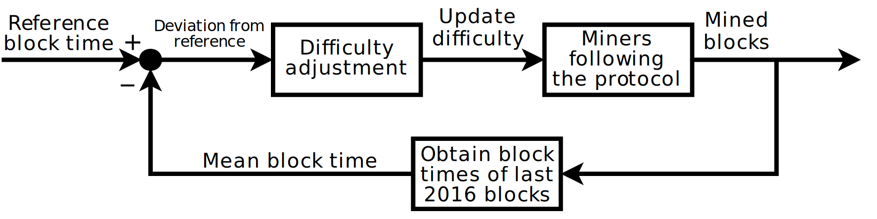
It is a feature of public blockchains, where a protocol parameter needs to adapt to certain conditions, but should not be controlled by a specific participant. The solution is to implement a mechanism where it auto-adjusts, according to quantifiable and objective conditions. The primary example is Bitcoin’s difficulty adjustment. There, variations in average block time are used to dynamically adjust Bitcoin’s block difficulty, every 2016 blocks. Owing to difficulty adjustment, Bitcoin blocks are mined every 10 minutes on average without any external control. Shifts in block time feed back into the difficulty parameter, which then dampens said shifts, creating a negative feedback loop. Here, Bitcoin makes use of elementary control theory, setting mean block time as a process variable and difficulty adjustment as the control action:

Gas Price Volatility

Unsharded blockchains have a limited supply, and a vertical supply curve. For that reason, blockchain resources are subjected to very high price volatilities, once user demand surpasses platform capacity.

For Ethereum, demand for gas isn’t distributed equally around the globe. Ethereum users exist in every inhabited continent, with the highest demand seen in East Asia, primarily China. Europe+Africa and the Americas seem to be on par in terms of demand. This results in predictable patterns that follow the peaks and troughs of human activity in each continent. The correlation between gas usage and price is immediately noticeable, demonstrated by a 5 day period from March 2019 (this is from a blog post of mine from last year).

The grid marks the beginnings of the days in UTC, and the points in the graph correspond to hourly averages, calculated as:

Average hourly gas usage per block = Total gas used in an hour / Number of blocks in an hour
Average hourly gas price = Total fees collected in an hour / Total gas used in an hour

Price oscillations are caused by the daily demand cycle. When we average out daily chunks of data, we obtain the following profiles:

To learn more about gas price volatility in Ethereum, see this blog post.

In EIP-1559, the feedback loop is set in a way to adjust an in-protocol price floor. This time, the process variable is block fullness. The price floor adjusts dynamically according to block fullness to ensure that demand at a given time does not exceed supplied blockchain throughput. The proposed mechanism does not aim to neutralize long term volatility though—it aims to discover the objective gas price, increase market efficiency and bring short-term stability to the gas price. The frequency of the control action is every 13~14 seconds (Ethereum’s block time), where the price can adjust by 1/8. For that reason, hour to hour and day to day volatilities remain. (Correct me if I’m wrong here)

What if we wanted the price to remain stable in the longer term, but also ensure that surges are infrequent enough not to affect the user experience?

Long-term Gas Price Adjustment

We consider a toy smart contract platform with constant block time. Here, we’ll try to implement a mechanism which stabilizes the gas price, but keeps congestion at bay at the same time. The control mechanism admits the following parameters:

CONTROL_RANGE: Number of blocks between two consecutive price adjustments.
TARGET_FULLNESS: The reference fullness value the mechanism should correct to.
INITIAL_PRICE: The initial value of the fixed gas price.
PRICE_ADJUSTMENT_RATE: The rate at which price increases or decreases after an adjustment.
BLOCK_GAS_LIMIT: The maximum amount of gas that can be used by transactions included in a block.

Once every CONTROL_RANGE blocks, the following algorithm updates the in-protocol fixed gas price:

# blocks: an array of the last CONTROL_RANGE blocks
# prev_price: previous fixed price

fullnesses = []
for b in blocks:
    fullnesses.append(b.get_gas_used()/BLOCK_GAS_LIMIT)

if median(fullnesses) > TARGET_FULLNESS:
    next_price = prev_price * (1 + PRICE_ADJUSTMENT_RATE)
else:
    next_price = prev_price / (1 + PRICE_ADJUSTMENT_RATE)

We believe that optimal values for above parameters exist, which can be found by a combination of simulations, econometrics and trial & error. Once set, we hope that the control mechanism can bring daily gas price stability to the blockchain.

Use Cases

Gas price action results from a combination of

the daily demand cycle,
long-term trends (e.g. ICO and DeFi bubbles), and
acute cases of hype (e.g. cryptokitties).

The most important use case is for a separate blockchain or an Ethereum shard, whose users demand that the gas price remains constant throughout the day. This neutralizes the volatility due to (1).

The demand can still shift slowly in the longer term, and the price floor would adapt accordingly. This accommodates the volatility due to (2).

However, since the adjustment rate is relatively slow—less than 10% per day—the mechanism will most likely not be able to accomodate the volatility due to (3), which can cause gas prices to increase 5-10x in a matter of days. For that reason, it would be wise to not just fix the price, but allow users to pay a premium on top of it.

Why would we want to neutralize (1)? The main argument is this: A business manifested as a dapp on Ethereum and takes on the transaction fees of its users via something like the Gas Station Network would like to have predictable operating expenses. They would like to be able to plan ahead, and not have to stop operation due to abnormally high fees. For them, any improvement in predictability is a plus. So they would be willing to pay more than the average user just to be able to keep a fixed cost per user in their accounting.

This means that the mechanism overprices gas, setting a barrier for the average user. This is necessary to dampen the daily demand cycle, because the price needs to be high enough, so that block space utilization is barely at capacity at the daily high. Using the mechanism this way would not only push certain users from the market, but also attract a different type of user—the type that values predictability as much as utility. Therefore, the blockchain/shard would end up in a different market position—one that we haven’t seen out in the wild until this point. One could say it would be an “exclusive” type of chain, with possibly less users than an unregulated chain, but at the same time with higher value.

Note that another volatility to consider is the price of ETH itself. If ETHUSD changes at a higher rate than the adjustment rate of the mechanism, then it would not be as effective. For that reason, one can imagine the mechanism using a price oracle, and setting and adjusting price in fiat terms. To be clear, transaction fees would still be paid in ETH; just that the gas price would be fixed in fiat terms through ETH, i.e. Gas <> ETH <> USD.

Simulations

The implementation of the simulations below can be found in this git repository.

Generating Demand

We treat the demand curve as a cumulative distribution function, and use inverse transform sampling to generate prices for the transactions submitted by users. We then verify our method by superimposing the histogram of sampled prices with the original demand curve:

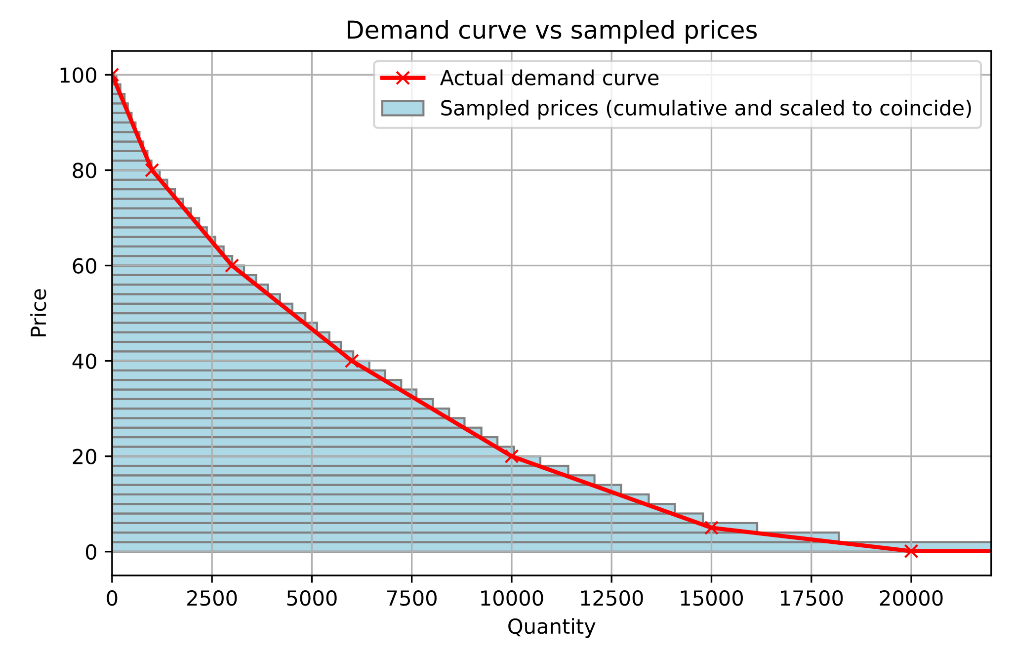
While simple, this method depends on the following assumption: Changes in demand are reflected by a shifting of the demand curve which doesn’t have to be uniform. The exact behavior of the demand curve is often complex, and simple models may fail to capture the nuances of a given market. In our method, increased demand reflects as a uniform scaling of demanded quantity with respect to a given price. E.g. in the figure above, changes in demand would cause the blue line to be scaled uniformly and vertically around the horizontal axis.

Modeling Number of Buyers (Users) per Block

Given a demand curve, we can sample as many prices as we want. To model the daily demand cycle realistically, we can use a certain model to set the number of available users in the market that bid for inclusion in a single block. Whether they would send a transaction or get it included would depend on

whether the price is floating or fixed,
and others’ transactions and gas prices.

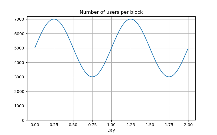
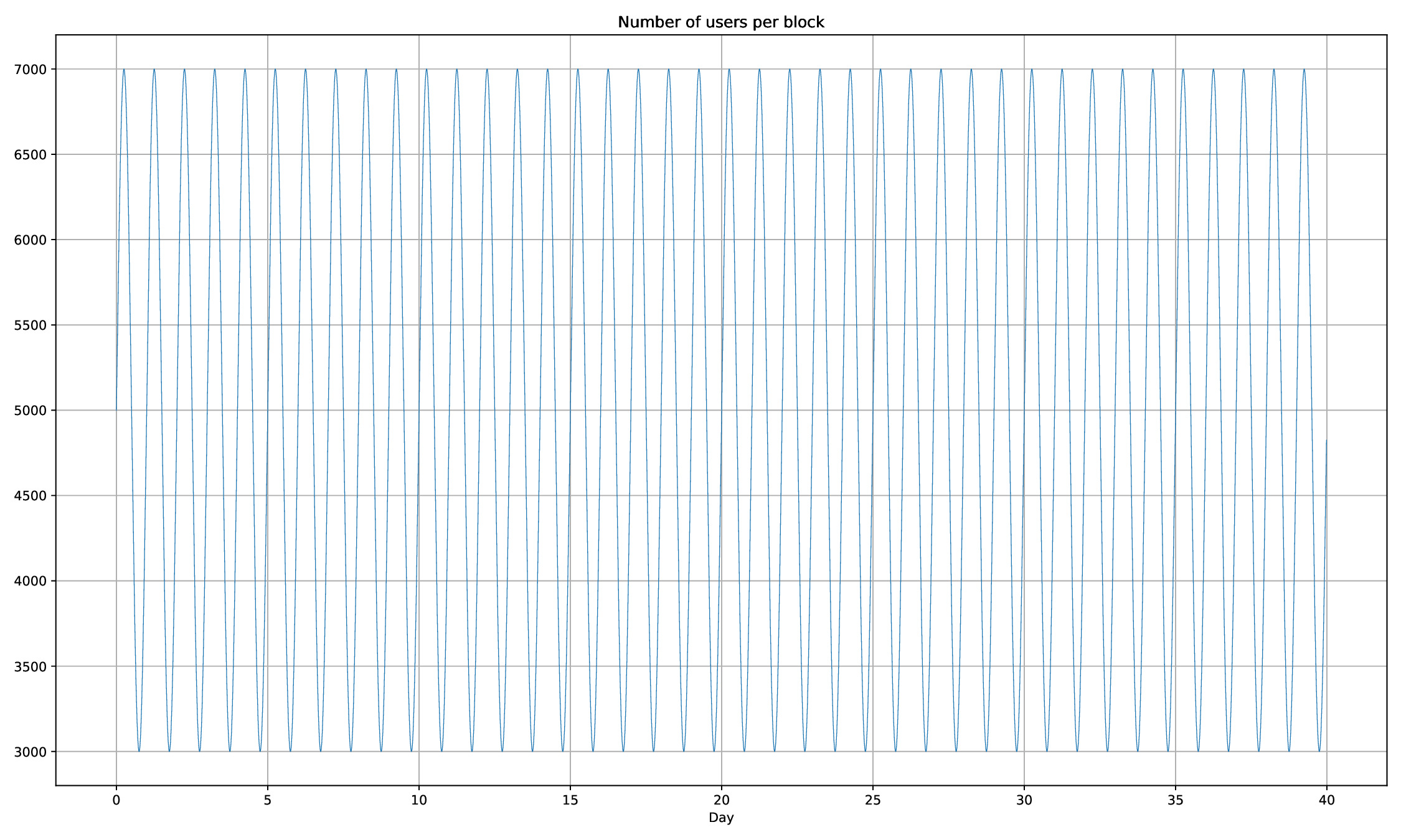
Below is a model which oscillates between 3000 and 7000 users per block.

Simulating a Floating Gas Price

We try to reproduce the daily demand cycle with a system that allows the gas price to float. Samples from the demand curve determine the willingness-to-pay (WTP) values of the agents. The agents then look at the minimum price of the previous block as a benchmark to determine how much they will set their gas price. By default, agents who can afford it overbid the previous block’s minimum price by a factor of OVERBIDDING_RATE.

If WTP <= min_price, they don’t submit a transaction, because they can’t afford to get it included.
If min_price <= WTP < min_price*(1+OVERBIDDING_RATE), they submit a transaction with WTP as the gas price.
If WTP >= min_price*(1+OVERBIDDING_RATE), they submit a transaction with min_price*(1+OVERBIDDING_RATE) as the gas price.

With this strategy, we can run a simulation and plot the median gas price from each block to see how it evolves. We let the initial price be relatively low, to see if it eventually converges to the market price:

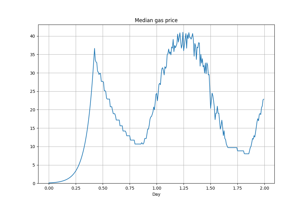
Here, most agents overbid in the first half of the first day, which results in an exponential trend, due to how they keep multiplying price with the same rate. The trend continues until some agents aren’t able to afford getting their transactions included in blocks, after which we see the prices mimic the curve we have given above.

Since the agents who can’t afford inclusion don’t submit transactions, we initially see a drop in the number of transactions submitted per block, which then converges to a stable value.

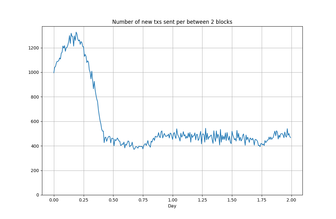
Indeed, it converges to around 476, the maximum number of transactions that can exist in a block.

Simulating Price Adjustment

We implement the price adjustment algorithm that we described above. This simulation is simpler than the floating price case in terms agent strategy, since agents have only one option: submit a transaction at the protocol enforced fixed gas price, or not, depending on whether they can afford it:

If WTP >= fixed_price, they submit a transaction.
Otherwise, they don’t submit a transaction.

We run the simulations with the following parameters:

BLOCK_GAS_LIMIT = 10_000_000
TX_GAS_USED = 21_000
BLOCK_TIME = 600
BLOCKS_IN_DAY = floor(SECONDS_IN_DAY / BLOCK_TIME)
CONTROL_RANGE = BLOCKS_IN_DAY
TARGET_FULLNESS = 0.65
PRICE_ADJUSTMENT_RATE = 0.01

Block time is 10 minutes, because simulations take too long otherwise. The first 2 parameters are taken from Ethereum, which result in 476 transactions per block. We set the control range as 1 day, target a median fullness of 65%, and allow the price to adjust 1% at a time.

We use the same function as before to generate the number of users per block, and let it run for 40 days:

We set the initial price to 35, and see if it converges to the market price we observed in the previous simulation:

It indeed converges to ~39, the maximum price we have observed in the previous simulation! This is because of the median fullness value we are targeting, 0.65, is selected to ensure that blocks are roughly 100% full during the height of the demand, with the current degree of daily volatility. This is indeed the case, once the price stabilizes:

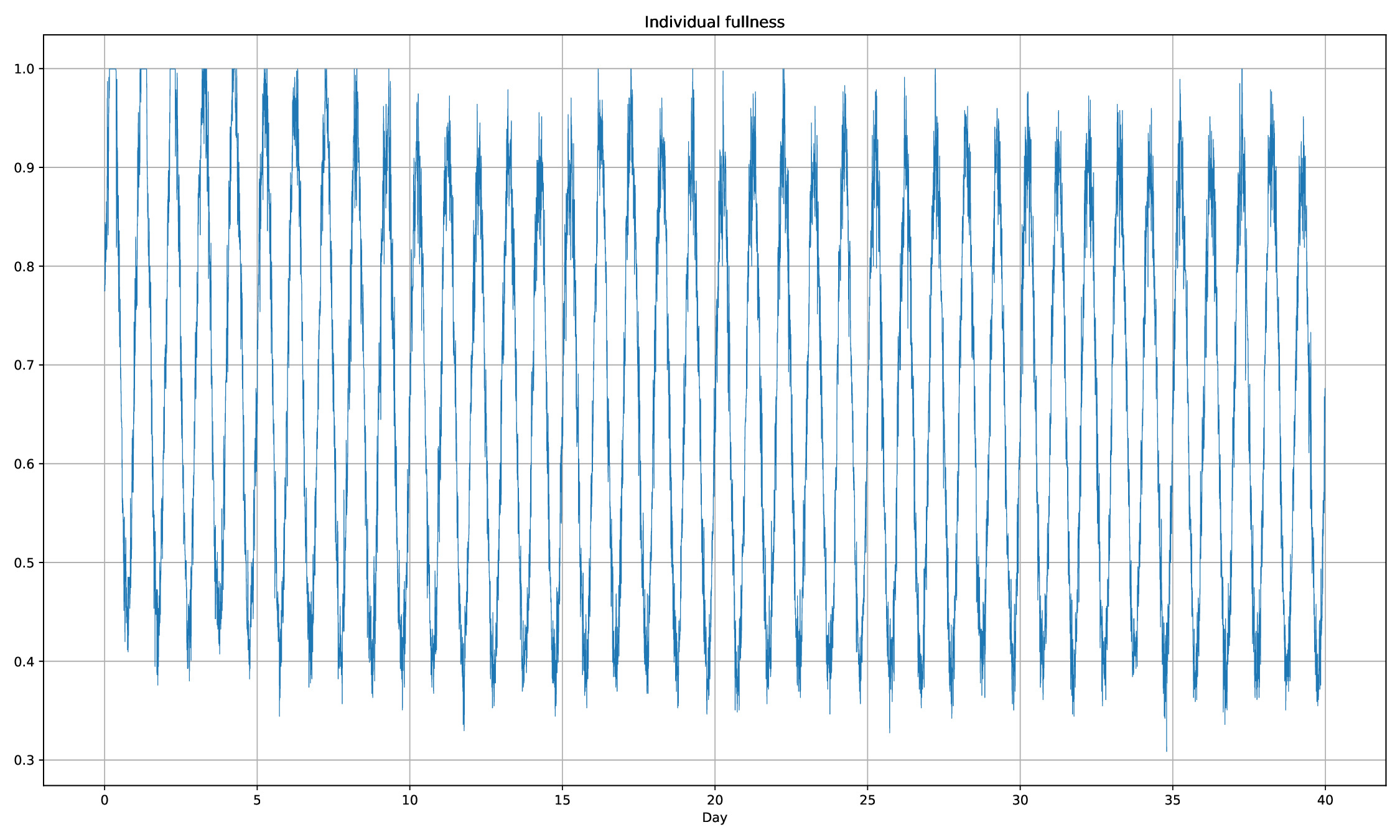
If we were to plot the process variable, we would see it converge to 0.65:

With price adjustment, transactions don’t wait in the transaction pool and immediately get included. If we plot the size of the transaction pool versus time, we should see it converge to zero once the price stabilizes:

There are a few days where a few transactions don’t get included immediately, but price adjustment did not claim to eliminate all surges in the first place. Price adjustment removes 99% of the surges, and during the remaining 1%, users would have to depend on the premium to prioritize transactions.

Price Adjustment during a Long-Term Trend

In the previous example, price adjustment successfully absorbed the daily volatility of our toy blockchain. However, we also wonder what would have happened if there were a long-term trend, superimposed with the daily cycle.

To answer the question, we use the following demand versus time curve:

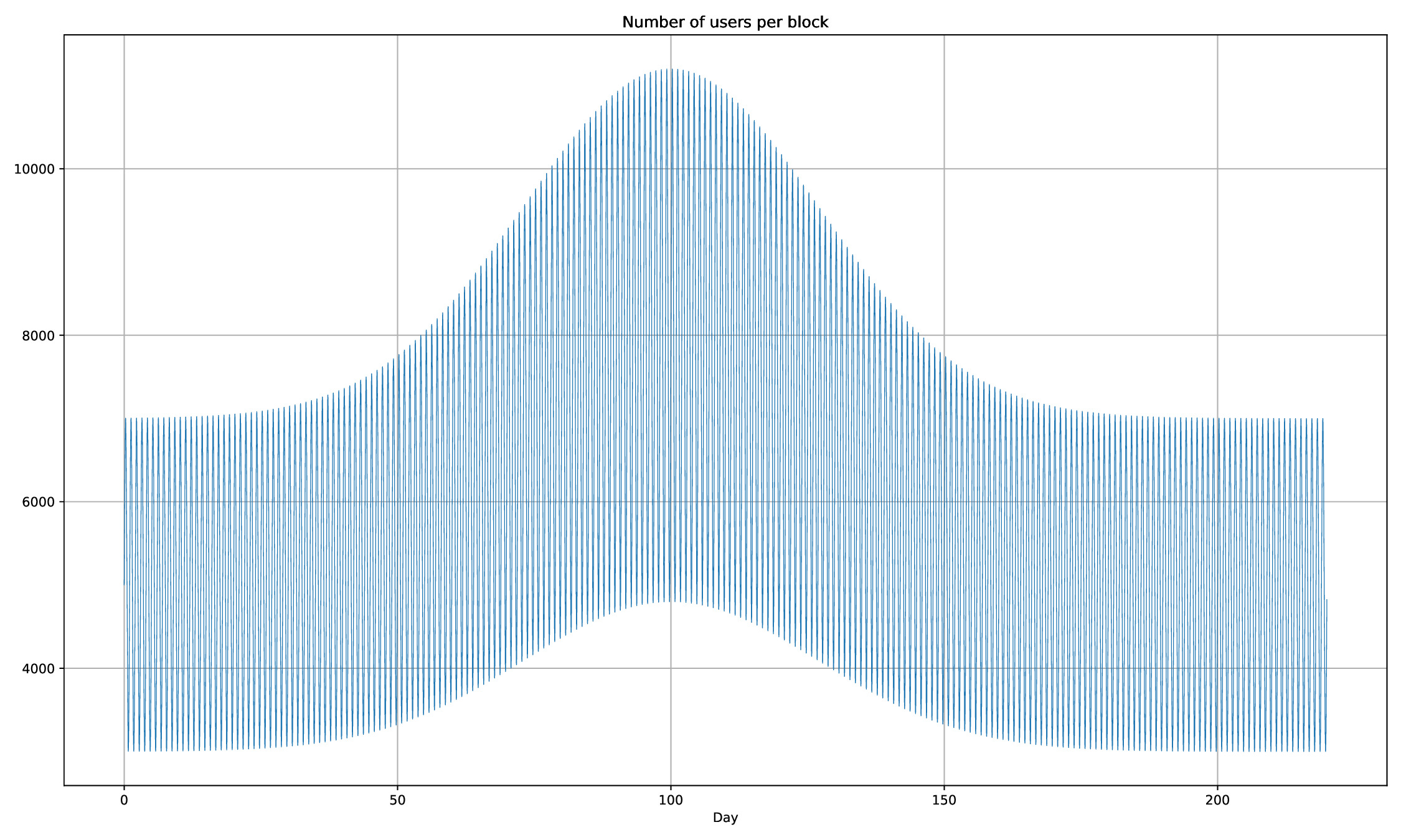
It’s the same cycle as before, but in the longer term, it increases until maximum height is reached around 100 days, and then decreases with the same rate.

We see that price evolves parallel to the trend:

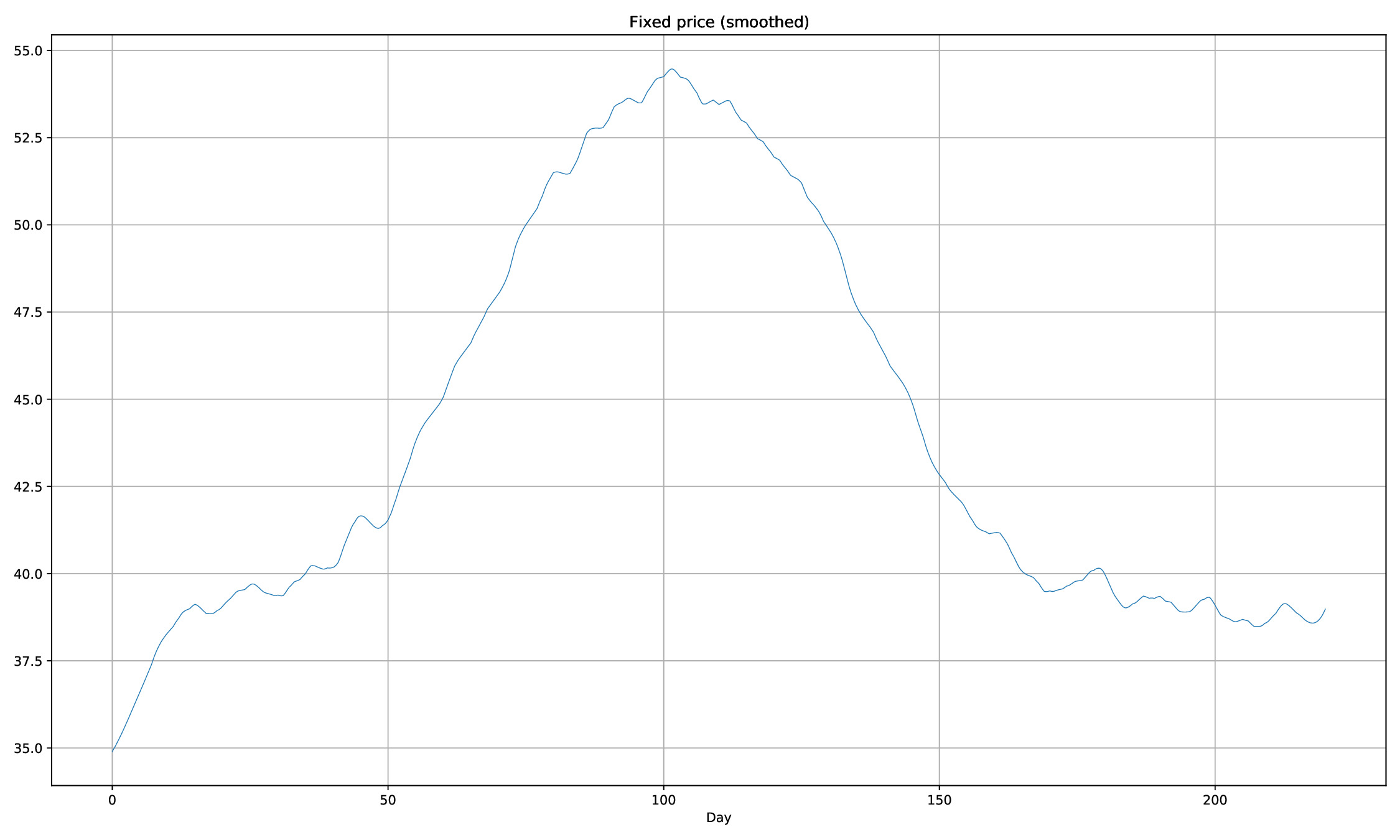
The price reaches a high of 54, after which it subsides and converges back to the usual 39. The important thing is, while we don’t observe volatility during the day, the gas price automatically adjusts to new market conditions without an external actor deciding for it.

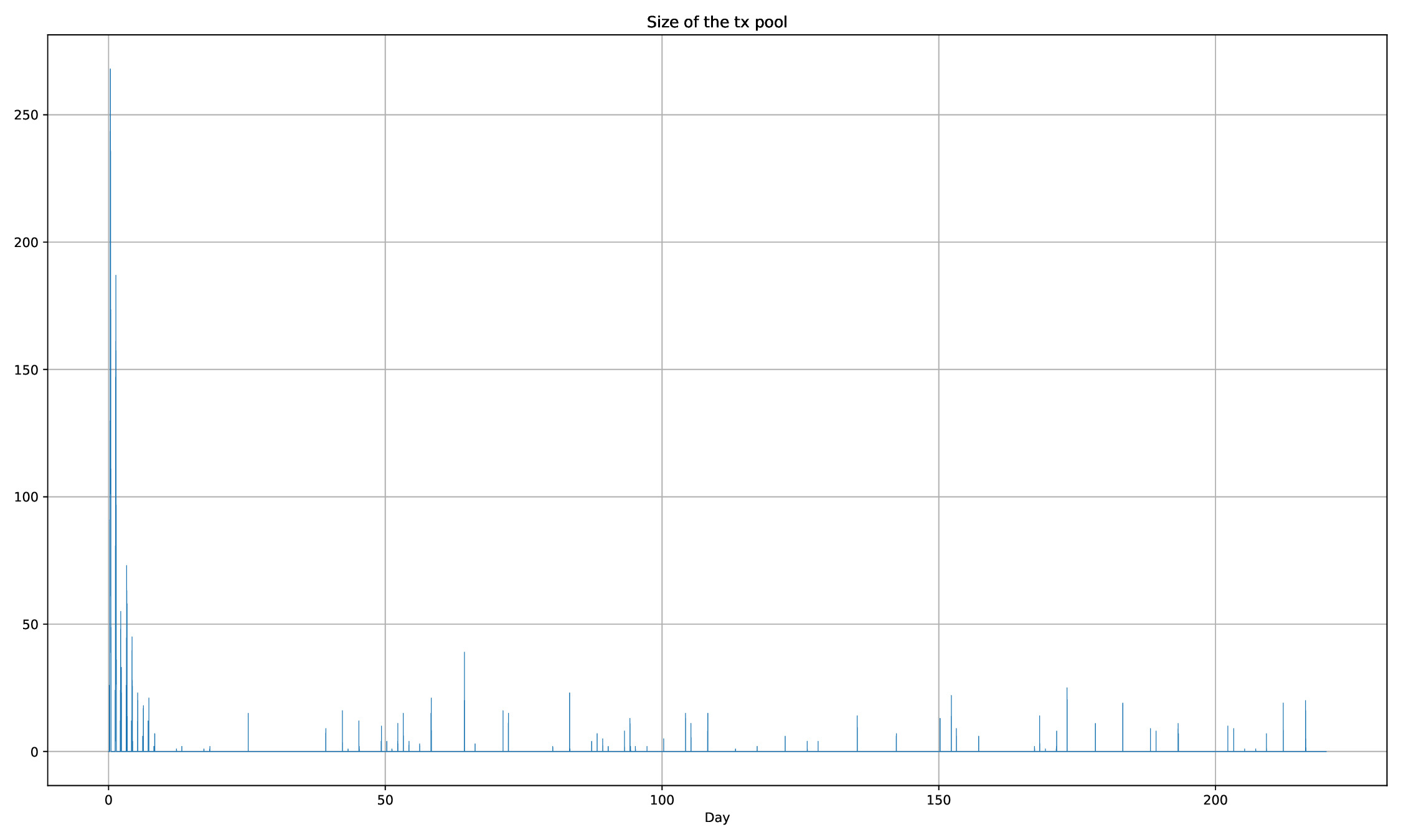
The size of the transaction pool shows us that price adjustment still prevents surges, even when there is a long-term trend with the demand.

Conclusion

We introduced a way for blockchain protocols to adjust prices of resources in a self-governing way, without the need for an external actor, and absorb most of the daily volatility. The mechanism uses block fullnesses as a process variable to adjust an in-protocol gas price. This eliminates short term surges, and allows the price to slowly adapt to new market conditions at the same time.

Future Work

Possible routes:

Calculate the evolution of the actual Ethereum demand curve using live txpool data.
Use the real life demand curve to test out the mechanism introduced above.
Extend the simulator and experiment with EIP-1559.