Authors: George Kadianakis <@asn>, Ansgar Dietrichs <@adietrichs>, Dankrad Feist <@dankrad>
In this work we demonstrate how to do amortized verification of multiple KZG multiproofs in the context of Data Availability Sampling. We also provide a reference implementation of our technique in Python.
Motivation
In Ethereum’s Data Availability Sampling design (DAS), validators are asked to fetch and verify the availability of thousands of data samples in a short time period (less than four seconds). Verifying an individual sample, essentially means verifying a KZG multiproof.
Verifying a KZG multiproof usually takes about 2ms where most of the time is spent performing group operations and computing the two pairings. Hence, naively verifying thousands of multiproofs can take multiple seconds which is unacceptable given Ethereum’s time constraints.
Furthermore, a validator is expected to receive these samples from the network in a streaming and random fashion. Hence, ideally a validator should be verifying received samples frequently, so that she can reject any bad samples, instead of just verifying everything in one go at the end.
The above two design concerns motivate the need for an amortized way to efficiently verify arbitrary collections of DAS samples.
Overview
In this work we present an equation to efficiently verify multiple KZG multiproofs that belong to an arbitrary collection of DAS samples. Our optimization technique is based on carefully organizing the roots of unity of our Lagrange Basis into cosets such that the resulting polynomials are related to each other.
We start this document with an introduction of the basic concepts behind Ethereum’s Data Availability Sampling. We also provide some results about KZG multiproofs and roots of unity.
We then present our main result, the Universal Verification Equation. After that and for the rest of the document, we provide a step-by-step account on how to derive the universal equation from first principles.
Throughout this document we assume the reader is familiar with the basics of Ethereum’s Data Availability Sampling proposal. We also assume familiarity with polynomial commitment schemes, and in particular with KZG multiproof verification and the Lagrange Basis.
Introduction to Data Availability Sampling
In this section we will give an introduction to Ethereum’s Data Availability Sampling logic. We start with a description of how the various data structures are organized, and we close this section with a simplified illustrative example.
DAS data format
In DAS, data is organized into blobs where each blob is a vector of 8192 field elements. The blob is mathematically treated as representing a degree < 4096 polynomial in the Lagrange Basis. That is, the field element at position i in the blob is the evaluation of that polynomial at a root of unity.
Blobs are stacked together into a BlobsMatrix which includes 512 blobs. For each blob, there is a KZG commitment that commits to the underlying polynomial.
Data Availability Sampling
For the purposes of DAS networking, each blob is split into 512 samples where each sample contains 16 field elements (512*16 = 8192 field elements). Hence a BlobsMatrix has 512 blobs and each blob is composed of 512 samples, which means that BlobsMatrix can be seen as a 2D matrix with dimensions 512x512.
Each sample also contains a KZG multiproof, proving that those 16 field elements are the evaluations of the underlying blob polynomial at the right roots of unity. Given a sample, a validator can verify its KZG multiproof against the corresponding blob commitment, to ensure that the data in the sample correspond to the right blob.
Every individual sample (along with its KZG multiproof) is then propagated over the network using gossip channels to interested participants. Validators are expected to fetch samples and validate two full rows and two full columns of the BlobsMatrix which corresponds to essentially verifying 2048 KZG multiproofs.
In the full DAS protocol we also use Reed-Solomon error-correction for the blob data but due to it being orthogonal to KZG verification it will be ignored for the rest of this document for the sake of simplicity. We will also avoid delving into the various design decisions of the DAS protocol that are not directly relevant to KZG verification.
Reverse Bit Ordering
In the blob’s Lagrange Basis, we carefully re-order the group of roots of unity of order 8192 in reverse bit ordering . This gives us the useful property that any power-of-two-aligned subset, is a subgroup (or a coset of a subgroup) of the multiplicative group of powers of \omega.
As an example, consider the group of roots of unity of order 8192: \{1, \omega, \omega^2, \omega^3, ..., \omega^{8191}\}. We use indices to denote the ordering in reverse bit order: \{\omega_0, \omega_1, \omega_2, \omega_3, ..., \omega_{8191}\} = \{1, \omega^{4096}, \omega^{2048}, \omega^{6072}, ..., \omega^{8191}\}. Then \Omega = \{\omega_0, \omega_1, \omega_2, ..., \omega_{15}\} is a subgroup of order 16, and for each 0 <= i < 512, we can use the shifting factor h_i = \omega_{16i} to construct the coset H_i = h_i \Omega.
The benefit of using reverse bit ordering in that way is that we ensure that all sequential chunks of size 16 in our Lagrange Basis correspond to different cosets of \Omega. This is crucial because samples are 16 field elements in Lagrange Basis and this ordering provides the important property that the evaluation domains of our samples are cosets of each other.
An illustrative example of a BlobsMatrix
For the purposes of demonstration, we present a simplifiedBlobsMatrix with four blobs representing four polynomials p_1, ... p_4. Each polynomial is represented as a vector of eight field elements in Lagrange Basis.
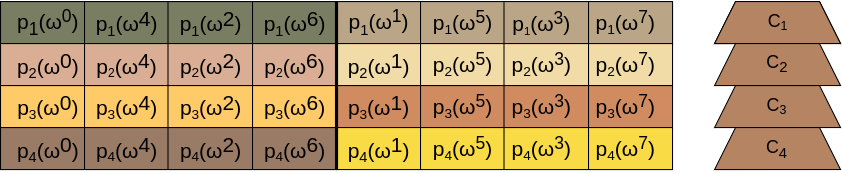
Each cell of the matrix corresponds to a field element in the Lagrange Basis. Each blob is split in two samples (color coded) with four field elements each.
On the right of each blob there is a commitment C_i that commits to the polynomial p_i.
We now make two important observations that we will use later:
- Each vertical slice of the matrix includes evaluations over the same root of unity.
- In each blob, each sample’s evaluation domain is a coset of the first sample’s domain. In our example, the evaluation domain of the second sample is a coset of the domain of the first sample with \omega^1 as its shifting factor (because of the reverse bit ordering).
The KZG multiproofs of the samples on the above matrix are not depicted for simplicity. However, here is an artistic depiction of the first sample of the first blob along with its multiproof:
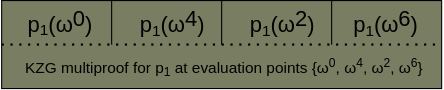
We would like to remind to the reader that in regular DAS, the BlobsMatrix above would have 512 blobs/rows. Each row would have 8192 vertical slices, representing 512 samples/columns with 16 field elements each, for a total number of 512*512=262144 samples. The sole sample depicted above would have 16 field elements at 16 different evaluation points which are defined by the reverse bit ordering.
Introduction to KZG multiproofs
A KZG multiproof [q(s)] proves that a polynomial p(x) with commitment C evaluates to (\nu_1, \nu_2, ..., \nu_n) at domain \{z_1, z_2, z_3, ..., z_n\}. That is, p(z_1) = \nu_1, p(z_2) = \nu_2 and so on.
Verifying a KZG multiproof involves checking the pairing equation below:
which effectively checks the following relationship of the exponents:
where
- q(x) is the quotient polynomial
- Z(x) is the vanishing polynomial
- p(x) is the commited polynomial
- I(x) is the interpolation polynomial
In the section below we delve deeper into the structure of the vanishing polynomial.
Vanishing polynomials
For a KZG multiproof with domain \{z_0, z_1, z_2, ..., z_{n-1}\} the vanishing polynomial is of the form Z(x) = (x-z_0)(x - z_1)(x - z_2)...(x- z_{n-1}).
We observe that if the domain is the group of n-th roots of unity \Omega = \{1, \omega, \omega^2, ..., \omega^{n-1}\} the vanishing polynomial simplifies to:
The above follows algebraically (try it out and use the properties of roots of unity to eventually see all terms canceling out) but also from the fact that the n-th roots of unity are the roots of the polynomial x^n -1.
Furthermore, if the domain is a coset of the roots of unity H_i = h_i \Omega, the vanishing polynomial becomes:
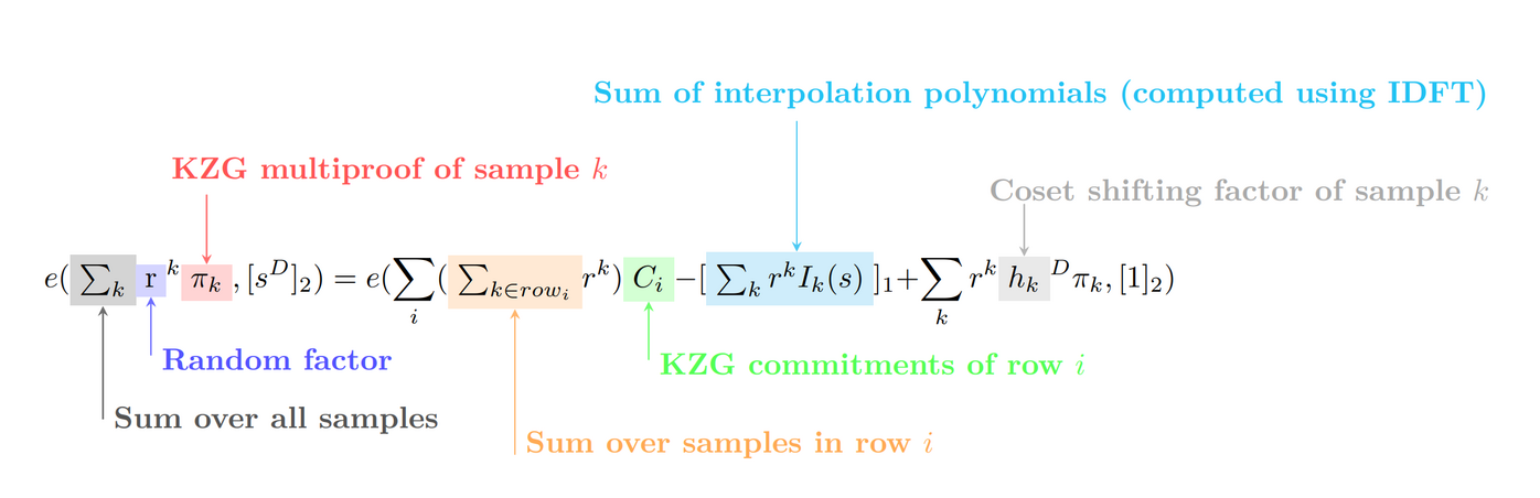
The Universal verification equation
As our main contribution, we present a universal equation to efficiently aggregate and verify an arbitrary number of DAS samples (and hence KZG multiproofs) regardless of their position in the BlobsMatrix.
We first present the equation in its full (and hideous) form, and then over the next sections we will derive it from scratch in an attempt to explain it.
We introduce the following notation that will also be used in later sections:
- k is an index for iterating over all samples we are verifying
- i is an index for iterating over the rows of the
BlobsMatrix - \pi_k is the KZG multiproof corresponding to sample k (i.e. [q_k(s)])
- D is the size of the cosets of roots of unity (D=16 in DAS)
- h_{k} is the coset shifting factor corresponding to sample k
- \text{row}_i is the set of samples we are verifying from row i of the
BlobsMatrix
Given the above notation, we derive the following verification equation:
or in annotated form:
Step-by-step derivation of the universal equation
In this section we will explore how the above equation came to be.
We first lay down some foundations on how we can aggregate multiple KZG multiproofs, and then break the process into pieces to derive the universal equation.
Naive approach
Given n KZG multiproofs \{[q_1(s)], [q_2(s)], .., [q_n(s)]\}, the direct verification approach needs to check the following equations:
Verifying the above using (M1) takes 2n pairing checks.
We can do this verification more efficiently by verifying the entire system of equations using a random linear combination with the powers of a random scalar r (for more information about this standard technique you can read the SnarkPack post or section 1.3 of the Pointproofs paper):
The above can be verified by evaluating at s using the following pairing equation:
The above equation is a decent starting point but suffers from a linear amount of pairings and is heavy on group operations.
What’s the game plan?
In the following sections we focus on optimizing individual parts of the above equation (K2).
In the section below we will reduce the number of pairing computations by grouping factors together.
In subsequent sections, we will reduce the number of group operations by replacing them with field operations which are an order of magnitude cheaper.
Amortizing pairings by aggregating vanishing polynomials
Let’s start on the left hand side of equation (K1):
This is particularly problematic because verifying the above sum in (K2) takes n pairings, where n is the number of samples we are verifying.
From the example above, we observe that the evaluation domain of samples are cosets of the roots of unity of size 16. This allows us to use result (V1) about vanishing polynomials as follows:
where D=16.
The above finally comes down to:
which can be evaluated at s using just two pairings:
The above simplification allows us to move from a linear amount of pairings to just two pairings. This represents a huge efficiency gain.
Amortizing group operations by aggregating interpolation polynomials
Now let’s focus on the right hand side of equation (K2) and in particular on the sum of the interpolation polynomials:
The way the sum is written here, we commit to each interpolation polynomial I_k(x) separately, and then sum up the [I_k(s)] commitments. This approach requires a linear amount of commitments, which are expensive to compute as they involve group operations.
Instead, we can compute the random linear combination \sum r^k I_k(x) of the individual interpolation polynomials first, and then calculate a single commitment to that aggregated polynomial:
In the appendix we provide instructions on how to efficiently calculate the random linear combination of the interpolation polynomials.
Amortizing group operations by aggregating commitments
Finally, let’s focus on the right hand side of equation (K2) and in particular on the sum of the commitments:
Let’s consider the case where multiple samples have the same polynomial p_k as is the case for samples on the same row. In that case, we can aggregate the random factors r^k, by iterating over every row and summing up the random factors of its samples as follows:
As a trivial example, consider that we are aggregating two samples from the same row, which both have corresponding commitment C. Instead of computing r_1C + r_2C, we can compute (r_1 + r_2)C, which gives us a big efficiency boost, since we replace one group operation with a field operation.
Bringing everything together
We are finally ready. Time to unite all pieces of the puzzle now!
We start with equation (K1):
We aggregate the vanishing polynomials using result (Z1) to get:
We turn it into a verification equation by evaluating at s and using result (Z2):
We can now merge the two last pairings using the bilinearity property:
Finally we apply result (C1) to aggregate the commitments over the rows to arrive at the final verification equation:
Efficiency analysis
The final verification cost when verifying n samples:
- Two pairings
- Three multi-scalar multiplications of size at most n (depending on the rows/columns of the samples)
- n field IDFTs of size 16 (to compute the sum of interpolation polynomials)
- One multi-scalar multiplication of size 16 (to commit to the aggregated interpolation polynomial)
The efficiency of our equation is substantially better than the naive approach of verification which used a linear number of pairings. Furthermore, using the interpolation polynomial technique we avoid a linear amount of multi-scalar multiplications and instead do most of those operations on the field. Finally, our equation allows us to further amortize samples from the same row by aggregating the corresponding commitments.
Reference Implementation
We have implemented our technique in Python for the purposes of demonstration and testing.
As a next step, we hope to implement the technique in a more efficient programming language so that it can provide us with accurate benchmarks of the verification performance.
Discussion
How to recover from corrupt samples on the P2P layer?
As mentioned in the motivation section, the purpose of our work is for validators to efficiently verify samples received from the P2P network.
A drawback of our amortized verification technique is that if a validator receives a corrupt sample with a bad KZG multiproof, the amortized verification equation will fail without revealing information about which sample is the corrupt one.
This behavior could be exploited by attackers who spam the network with corrupt samples in an attempt to disrupt the validator’s verification.
While such P2P attacks are out-of-scope for this work, we hope that future research will explore validating strategies in this context. We believe that by sizing the verification batches and using bisection techniques like binary search, the evil samples can be identified and malicious peers can be flagged in the P2P peer reputation table of the validator so that they get disconnected and blacklisted.
Appendix
Details on aggregating interpolation polynomials
In a previous section we amortized the sum of the interpolation polynomials \sum r^k[I_k(s)] by aggregating the individual polynomials:
But how do we calculate this sum? An incorrect approach could have been to sum all the interpolation polynomials directly in the Lagrange Basis. This is not possible because samples from different columns contain field elements that represent evaluations at different evaluation points and hence they cannot be added naively in Lagrange Basis.
However, this also means that we can do a partial first aggregation step directly in the Lagrange Basis for samples from the same column (since those share the same evaluation domain):
After this partial column aggregation, we perform a change of basis from Lagrange basis to the monomial basis for every I_j(x) polynomial so that we can add those polynomials in (P1).
For this change of basis, we suggest the use of field IDFTs adjusted to work over cosets. We then also present a slightly less efficient alternative method without IDFTs.
Primary method: IDFTs over cosets
A change of basis from the Lagrange basis to the monomial basis can be done naturally with IDFTs over the roots of unity. However, in our use case, the evaluation domains of our interpolation polynomials are not the roots of unity but are instead cosets of the roots of unity.
We can show that for an interpolation polynomial with a coset of the roots of unity as its evaluation domain, we can perform the IDFT directly on the roots of unity, and then afterwards scale the computed coefficients by the coset shifting factor. We present an argument of why this is the case in a later section of the appendix.
More specifically, for a polynomial with a vector of evaluations \vec{\nu}, if its evaluation domain is a coset of the roots of unity with shifting factor h, we can recover its vector of coefficients \vec{c}, by first calculating \vec{c} = IDFT(\vec{\nu}) and then multiplying every element of \vec{c} by h^{-j} (where j is the index of the element in \vec{c}).
Using the above technique, we can compute (P1) by adding all the interpolation polynomials in monomial basis efficiently and finally doing a single commitment of the resulting polynomial in the end.
This strategy allows us to avoid the linear amount of commitments which involve group operations. Instead we get to do most computations on the field using IDFTs and finish it off with a single commitment operation in the end.
In the following section we will show an alternative approach of computing the interpolation polynomial sum.
Alternative method: avoiding IDFTs
As an alternative approach, verifiers can avoid implementing the complicated part of the IDFT algorithm at the cost of worse performance. In terms of performance, the change of basis for each sample will cost \mathcal{O}(n^2) field operations instead of \mathcal{O}(N*log N) but with n=16 this might be acceptable.
Our aim is to change the basis of our interpolation polynomials without doing a full fledged FFT. We want a direct way to go from the evaluations that can be found in the samples to the coefficients of the interpolation polynomials so that we can sum them together in (P1).
We will make use of the fact that the IDFT algorithm provides us with a direct formula for computing the coefficients of a polynomial given its evaluations over a multiplicative subgroup (in our case the subgroup of roots of unity of order D):
where:
- p^{(j)} is the j-th coefficient of polynomial p(x) of degree D
- \nu_l is the evaluation of p(x) at \omega^l
Unfortunately, like in the IDFT section above, we cannot use the above formula directly because the evaluation domains of our interpolation polynomials are not multiplicative subgroups but are instead cosets of multiplicative subgroups.
In such cases we can use a related formula (which is motivated in the last section of the appendix):
With the above formula in hand, we circle back to our original problem and look at the interpolation polynomial of a sample k in the monomial basis:
We don’t know the coefficient j of I_k(x), but using result (A2) we can express it in terms of its evaluations:
where:
- \nu_{k,l} is the l-th evaluation of I_k(x)
- h_k is the coset shifting factor of sample k
We can now use the above to calculate the final sum of interpolation polynomials:
By rearranging the sums we can turn this into a single polynomial:
Finally, commiting to (A3) gives us the desired result \sum r^k[I_k(s)] without ever running the full IDFT algorithm.
Perfoming IDFTs over cosets of roots of unity
We show that for a polynomial p(x) with a coset of a subgroup as its evaluation domain, we can perform an IDFT on the subgroup itself, and then afterwards scale the computed coefficients by the coset shifting factor.
We show this by constructing a new polynomial p'(x) with the following properties:
- The evaluation domain of p'(x) is the subgroup of roots of unity
- The evaluations of p'(x) at its evaluation domain are known
- The coefficients of p'(x) are trivially related to the coefficients of p(x)
Since the evaluation domain of p'(x) is the subgroup of roots of unity, and we know its evaluations, we can perform an IDFT on it to recover its coefficients and then scale them to recover the coefficients of p(x).
We construct p'(x) as follows:
such that p'(x) has the propety that p(h \omega) = p'(\omega) since:
Observe that p'(x) has the same evaluations as p(x) (which are known) but its evaluation domain is the subgroup of roots of unity (instead of a coset).
This allows us to perform the IDFT on p'(x) over the roots of unity to get its coefficients, and then use (A4) to scale the coefficients by the coset shifting factor to get the coefficients of p(x).