Many thanks to Alex, Csaba, Dmitry, Mikhail and Potuz for fruitful discussions and write-up review
Abstract
The present DAS approach for Ethereum is based on Reed-Solomon erasure coding + KZG commitments. The novel scheme (described here Faster block/blob propagation in Ethereum by @potuz) introduces another pair: RLNC (Random Linear Network Coding) erasure coding + Pedersen commitments. It has nice properties which could be used to consider an alternative Data Availability approach.
The protocol outlined in this write-up primarily sketches what an RLNC-based Data Availability design might look like. The concepts used here are still not sufficiently checked, let alone formally proved. In any case if these concepts turn out to be correct, the algorithm could serve as a foundation for prototyping. If some of them turn out to be incorrect, we can either adjust the algorithm or think about adjusting or replacing them.
The reasoning in this write-up overlaps at several points with that of @Csaba’s recent post: Accelerating blob scaling with FullDASv2 (with getBlobs, mempool encoding, and possibly RLC).
To explore the full context, including reasoning and discussion comments, see the extended version of this write-up: Alternative DAS concept based on RLNC - HackMD
Intro
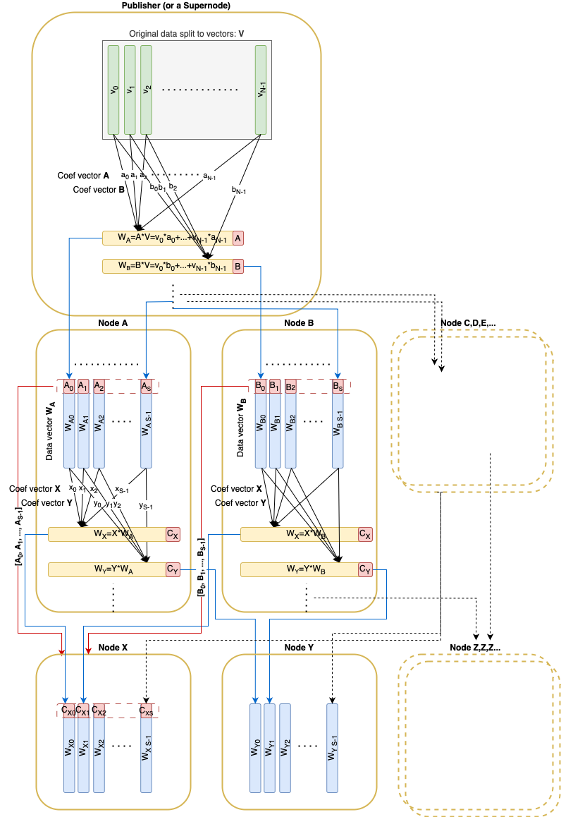
Much like the write-up Faster block/blob propagation in Ethereum, the original data is split into N vectors v_1, \dots, v_N over the field \mathbb{F}_p. These vectors can be coded using RLNC and committed via a Pedersen commitment (of size 32 \times N) included in the block. Any linear combination can be verified given the commitment and its associated coefficients.
We also assume that the coefficients may come from a much smaller subfield \mathbb{C}_q, whose size could be as small as a single byte—or even a single bit (DISCLAIMER: from the latest discussions it’s not confirmed that we may have secure EC over a field with such a smaller subfield).
Let’s also introduce the sharding factor S: any regular node needs to download and custody 1/S of the original data size.
Having a fixed shard factor S let’s take the total number of original vectors N = S^2
Brief protocol overview
A Pedersen commitment (size 32*N) is published in the corresponding block.
During dissemination each node receives pseudo-random linear combination vectors from its peers.
- this algorithm describes a non interactive approach where random coefficients are derived deterministicaly from the receiver’s
nodeIdand theRREFmatrix trick is used (DISCLAIMER: theRREFtrick isn’t strictly proved to work securely however there is an example which could be the proof starting idea) - there is also an available fallback option: an interactive approach where the responder first reveals its source coefficients, and the requester then requests the linear combination using locally generated random coefficients.
Every sent linear combination vector is accompanied by basis vectors of the subspace this vector was randomly sampled from. These basis vectors must form a matrix in RREF form. This condition ensures that the remote peer indeed possesses basis vectors for the claimed subspace.
The node continues sampling until both of the following conditions are met:
- All received basis vectors span the full N-dimensional space
- At least S vectors for custody have been received
After that, the node completes sampling and becomes an ‘active’ node, which can be used for sampling by other nodes.
Note
The below Python-like code snippets are for illustration purposes only, they are not intended to be compiled and executed for now. Some obvious or library-like functions lack their implementations so far.
Types
Let data vector elements be from a finite field \mathbb{F}_p which could roughly be mapped to 32 bytes
type FScalar
Let coefficients \mathbb{C}_q be from a subfield of (or equal to) \mathbb{F}_p
type CScalar
Let a single data vector has VECTOR_LEN elements from \mathbb{F}_p
type DataVector = Vector[FScalar, VECTOR_LEN]
Let the whole data be spit onto N original DataVectors:
type OriginalData = Vector[DataVector, N]
Derived DataVector is a linear combination of original DataVectors. Since an original vector is just a special case of a derived vector we will no longer make any distinctions between them.
To validate a DataVector against commitment its linear combination coefficients should be known:
type ProofVector = Vector[CScalar, N]
There is also a slightly different sequence of coefficents which is used when deriving a new vector from existing DataVectors:
type CombineVector = List[CScalar]
Structures
A data vector accompanied by the its linear combination coefficients
class DataAndProof:
    data_vector: DataVector
    proof: ProofVector
The only message for dissemination is
class DaMessage:
    data_vector: DataVector
    # coefVector for validation is derived
    orig_coeff_vectors: List[CombineVector]
    seq_no: Int
There is an ephemeral store for a block data:
class BlockDaStore:
    custody: List[DataAndProof]
    sample_matrix: List[ProofVector]

    # commitment is initialized first from the corresponding block
    commitment: Vector[RistrettoPoint]
Functions
Let the function random_coef generates a deterministically random coefficient vector with the seed (nodeId, seq_no):
def random_coef(node_id: UInt256, length: int, seq_no: int) -> CombineVector
Let’s define utility functions to compute linear combinations:
def linear_combination(
        vectors: Sequence[DataVector],
        coefficients: CombineVector) -> DataVector
def linear_combination(
        vectors: Sequence[ProofVector],
        coefficients: CombineVector) -> ProofVector
Function which performs linear operations on DataVectors and ProofVectors simultaneously to transform the ProofVectors to RREF:
def to_rref(data_vectors: Sequence[DataAndProof]) -> Sequence[DataAndProof]
def is_rref(proofs: Sequence[ProofVector]) -> bool
The function creating a new deterministically random message from existing custody vectors for a specific peer:
def create_da_message(
        da_store: BlockDaStore
        receiver_node_id: uint256,
        seq_no: int) -> DaMessage:
    rref_custody = to_rref(da_store.custody)
    rref_custody_data = [e.data_vector for e in rref_custody]
    rref_custody_proofs = [e.proof for e in rref_custody]
    rnd_coefs = random_coef(receiver_node_id, len(rref_custody), seq_no)
    data_vector = linear_combination(rref_custody_data, rnd_coefs)
    return DaMessage(data_vector, rref_custody_proofs, seq_no)
Computes the rank of data vectors’ coefficients. The rank equal to N means that the original data can be restored from the data vectors.
def rank(proof_matrix: Sequence[ProofVector]) -> int
Publish
The publisher should slice the data to vectors to get OriginalData.
Before propagating the data itself publisher should calculate Pedersen commitments (of size 32 * N), build and publish the block containing these commitments.
Then the publisher should populate custody with data vectors (original) and their ‘proofs’ which are simply elements of a standard basis: [1, 0, 0, ..., 0], [0, 1, 0, ..., 0]:
def init_da_store(data: OriginalData, da_store: BlockDaStore):
    for i,v in enumerate(data):
        e_proof = ProofVector(
            [CScalar(1) if index == i else CScalar(0) for index in range(size)]
        )
        da_store.custody += DataAndProof(v, eproof)
Publishing process is basically the same as the propagation process except the publisher sends by S messages to a single peer in a single round instead of sending just 1 message during propagation.
def publish(da_store: BlockDaStore, mesh: Sequence[Peer]):
    for peer in mesh:
        for seq_no in range(S):
            peer.send(
                create_da_message(da_store, peer.node_id, seq_no)
            )
Receive
Assuming that the corresponding block is received and the BlockDaStore.commitment is filled prior receiving a message: DaMessage
Derive the ProofVector from original vectors:
def derive_proof_vector(myNodeId: uint256, message: DaMessage) -> ProofVector:
    lin_c = randomCoef(
        myNodeId,
        len(message.orig_coefficients),
        message.seq_no)
    return linear_combination(message.orig_coefficients, lin_c)
Validate
The message first validated:
def validate_message(message: DaMessage, da_store: BlockDaStore):
    # Verify the original coefficients are in Reduced Row Echelon Form
    assert is_rref(message.orig_coefficients)
    # Verify that the source vectors are linear independent
    assert rank(message.orig_coefficients) == len(message.orig_coefficients)
    # Validate Pedersen commitment
    proof = derive_proof_vector(my_node_id, message)
    validate_pedersen(message.data_vector, da_store.commitment, proof)
Store
Received DataVector is added to the custody.
The sample_matrix is accumulating all the original coefficients and as soon as the matrix rank reaches N the sampling process is succeeded
def process_message(message: DaMessage, da_store: BlockDaStore) -> boolean:
    da_store.custody += DataAndProof(
        message.data_vector,
        derive_proof_vector(my_node_id, message)
    )
    da_store.sample_matrix += message.orig_coefficients
    is_sampled = N == rank(da_store.sample_matrix)
    return is_sampled
is_sampled == true means that we are [almost] 100% sure that our peers who sent us messages collectively posses 100% of information to recover the data.
Propagate
When the process_message() returns True, this means that the sampling was successful and the custody is filled with enough number of vectors. From now the node may start creating and propagating its own vectors.
We are sending a vector to every peer in the mesh which didn’t sent any vector to us yet:
# mesh: here the set of peers which haven't sent any vectors yet
def propagate(da_store: BlockDaStore, mesh: Sequence[Peer]):
    for peer in mesh:
            peer.send(
                create_da_message(da_store, peer.node_id, 0)
            )
Feasibility
Let’s overview some numbers depending on S and |\mathbb{C}_q| (size of coefficients) assuming original data size of 32Mb:
| S | sizeOf(C) (bits) |
N = S^2 | Vector Size (Kb) | Commitment Size (Kb) | Msg coefs size (Kb) | Msg Overhead (%%) |
|---|---|---|---|---|---|---|
| 8 | 1 | 64 | 512 | 2 | 0.0625 | 0.01% |
| 8 | 8 | 64 | 512 | 2 | 0.5 | 0.10% |
| 8 | 256 | 64 | 512 | 2 | 16 | 3.13% |
| 16 | 1 | 256 | 128 | 8 | 0.5 | 0.39% |
| 16 | 8 | 256 | 128 | 8 | 4 | 3.13% |
| 16 | 256 | 256 | 128 | 8 | 128 | 100.00% |
| 32 | 1 | 1024 | 32 | 32 | 4 | 12.50% |
| 32 | 8 | 1024 | 32 | 32 | 32 | 100.00% |
| 32 | 256 | 1024 | 32 | 32 | 1024 | 3200.00% |
| 64 | 1 | 4096 | 8 | 128 | 32 | 400.00% |
| 64 | 8 | 4096 | 8 | 128 | 256 | 3200.00% |
| 64 | 256 | 4096 | 8 | 128 | 8192 | 102400.00% |
According to these numbers it’s basically not feasible to use this algorithm with S \ge 64. If there are no options to use small coefficients (1 or 8 bits), then S = 8 is the maximum sharding factor that makes sense due to the coefficient size overhead. (With S = 16, the minimal node download throughput would be the same as with S = 8.)
Pros and Cons
Pros
- The total data size to be disseminated, custodied and sampled is x1 (+ coefficients overhead which can be small if small coefficients are available) of the original data size (compared to x2 for PeerDAS and x4 for FullDAS)
- We potentially may have ‘shard factor’ S as large as 32 (or probably even greater with some other modifications to the algorithm), which means every node needs to download and custody just 1/S of the original data size. (v.s. 1/8 in the present PeerDAS approach: 8 columns from 64 original)
- Data is available and can be recovered by having just any S regular honest nodes successfully performed sampling
- Sampling can be performed having any S regular nodes (comparing to present DAS where a sampling node needs a variety of peers from distinct DAS subnets)
- The approach ‘what you sample is what you custody and serve’ (like PeerDAS subnet sampling but unlike full sharding peer sampling). The concerns regarding peer sampling approach described here
- Since no column slicing is involved separate blobs may just span several original data vectors and thus sampling process may potentially effectively benefit from EL blob transaction pool (aka
engine_getBlobs()) - No smaller subnets which may be vulnerable to sybil attacks
- Duplication of data on the transport level could potentially be lower due to the fact that a node needs S messages from any peers and the usage of RLNC coding
- RLNC + Pedersen could be less resource consuming than RS + KZG
Cons
- Commitment and proof size grow quadraticaly with sharding coefficient S.
- If smaller coefficients are not available (not proved to be secure) then just S=8 is feasible.
- Still need to estimate dissemination latency as a node may propagate data only after it completes its own sampling
- For happy case the minimal number of peers for sampling is 32 (comparing to 8 in PeerDAS)
Statements to be proved
The above algorithm relies on a number of [yet fuzzy] statements which need to be proved so far:
- A valid linear combination with requested random coefficients returned by a super-node proves that the responding node has access to the full data (enough vectors to recover). This statement doesn’t look that tricky to prove
- If a full-node claims it has basis vectors which form a coefficient subspace, then if a node requests a random vector from this subspace and get a valid data vector then it proves the responding node indeed has the basis vectors for the claimed subspace. The proof could be a generalization of the statement (1)
- An EC over \mathbb{F}_p with subfield \mathbb{C}_2 makes sense and is secure. (this doesn’t seem to be true according to the latest discussions)
- The trick with RREF basis form for zero-RRT sampling actually works.
(this example can give some intuition about the validity of this statement) - The described algorithm yields evenly distributed basis vectors across hones nodes for the full
N-dimensional space. There a pretty smallE(kind of 1-3) such that the rank of basis vectors of any randomly selectedS + Enodes would beNwith some ‘very high’ probability . The same should be true in a Byzantine environment