Acknowledgement: This is a joint work with Emanuele Viterbo and Dankrad Feist and is supported by ESP Grant FY24-1745 titled “Improvements to 2D Reed-Solomon Codes in DAS”.
In this post, we describe how block circulant (BC) codes can serve as an alternative to one-dimensional (1D) and two-dimensional (2D) Reed–Solomon (RS) codes in the Ethereum PeerDAS protocol. We present efficient encoding and reconstruction algorithms for BC codes, developed within the same implementation framework as the respective 1D RS algorithms. The proposed encoding algorithm also permits a graceful integration of KZG commitment scheme. We evaluate and compare the performance of BC codes in terms of code rate, stopping rate, and the size of the local codes they contain, against both 1D and 2D RS codes. A longer version of this post is available in SVF2026.
Block Circulant Codes
Block circulant (BC) codes are introduced in SVD2025 as a viable alternative to both 1D (currently used) and 2D RS codes (expected to be incorporated later) in PeerDAS. Similar to the 2D RS code, the BC code contains multiple local codes, and each local code can be designed as a [(n_0,k_0),D] stacked 1D RS code. By stacked 1D RS code, we mean a [n_0D ,k_0D] RS code whose codewords are stacked in D horizontal rows each row of length n_0, and k_0 columns representing information symbols). Therefore, it is compatible with the KZG scheme. It turns out that BC codes achieve certain operating regimes of rate, stopping rate and local code size that are not feasible with either a 1D or a 2D RS code.
In a 2D RS code, the symbols are arranged in a two-dimensional square grid and there are linear constraints binding symbols belonging to every row or column. In the case of a BC code, symbols are arranged on a circle and the circle is divided into multiple overlapping arcs. Every arc has two neighbouring overlapping arcs, one on the left and the other on the right assuming a clockwise direction. Symbols belong to every arc are subject to a set of linear constraints. We present a more concrete description in the next subsection.
A Description of the BC Code
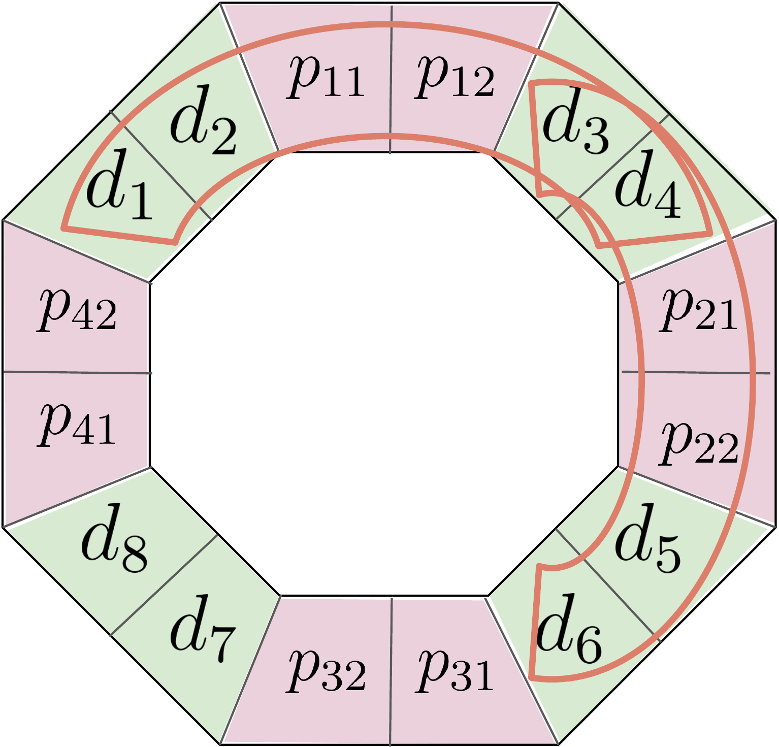
Figure 1: Illustration of the block circulant code. In this example, information symbols in the green background color are combined with parity symbols in the pink background color region resulting in the final arrangement. The groupings of symbols within the closed curves indicate local codes.
Consider the example consisting of n=16 symbols as given in Figure 1. There are \mu=4 arcs (two of them marked by closed curves) each containing n_0=6 symbols, equally spaced on the circle. There are a total of k=8 unconstrained symbols denoted as d_1, \ldots, d_8. Each local code contains k_0=4 unconstrained symbols. The remaining symbols are generated subject to certain linear constraints. In every arc, \rho=n_0-k_0=2 redundant symbols are added in such a manner that the local code corresponding to the arc becomes a 1D RS code. For example, the vector of symbols (d_1,d_2,p_{11},p_{12},d_3,d_4) corresponding to a single arc forms a codeword of an 1D RS code. Thus an arc is uniquely identified with a local code, and we may write arc and local code interchangeably. There lies exactly \omega=2 symbols at the overlapping region of two adjacent local codes and therefore we call \omega as the overlap width. Every unconstrained symbol is part of two distinct local codes and we call it the overlapping factor, denoted by \lambda. In the present arrangement, we have \lambda=2. In the general BC code presented in SVD2025, arrangements with higher values of \lambda are possible. Other parameters like \omega and \rho can also be modified suitably. It is shown in SVD2025 that a BC code with \lambda=2,3, the total number of erasures that can recovered by the BC code has been shown to be \lambda\rho. The ratio of total number of tolerable erasures to n is called the stopping rate and is denoted by S. We summarize the notations used for adjustable parameters of the BC code in the table below.
Parameters of BC code
| Notation | Meaning of the parameter(s) |
|---|---|
| \mu | Number of local codes |
| \lambda | Overlap factor (Every symbol is part of \lambda local codes) |
| \rho | Number of redundant symbols in a local code |
| \omega | Overlap width (Number of symbols two adjacent local codes overlap on) |
| [n_0,k_0]=[\lambda\omega+\rho,\lambda\omega] | Local code blocklength and dimension |
| [n,k]=[\mu(\omega+\rho),\mu\omega] | Global code blocklength and dimension |
| R=\frac{\omega}{\omega+\rho} | Rate |
| S=\frac{\lambda\rho}{\mu(\omega+\rho)} | Stopping rate |
| R_0=\frac{\lambda\omega}{\lambda\omega+\rho} | Local code rate |
| S_0=\frac{\rho}{\lambda\omega+\rho} | Local code stopping rate |
Stacked BC code
The procedure to convert an 1D RS code to stacked 1D RS code is described in detail in WZ2024. The exact procedure is applicable to the BC code as well because (a) each of the local code in the BC code is an 1D RS code, (b) the encoding can be performed by a series of local 1D RS encoders with carefully chosen set of evaluation points for each of the local code. We will describe the encoding procedure for a stacked BC code with the help of an example.
Encoding Algorithm
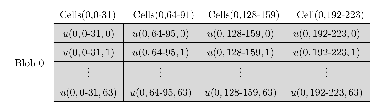
Figure 2 Structure of blob 0 before encoding.
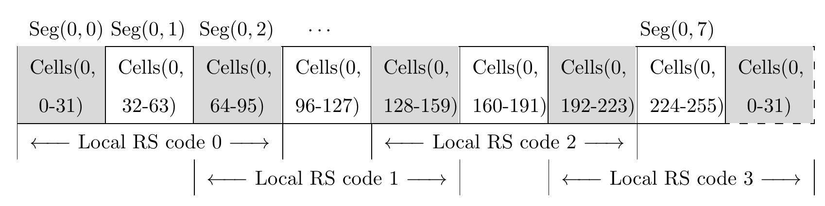
Figure 3 Structure of extended (encoded) blob 0 in BC code.
We describe the encoding with the help of an example illustrated in Figure 2 and 3. Here, overlap factor \lambda=2 and there are \mu=4 local codes. We pick the stacking parameter D=64 and a blob consists of 8192 finite field symbols arranged in k=128 cells. Each blob is an element of \mathbb{F}_q^{(D \times k)}=\mathbb{F}_q^{(64 \times 128)}, whereas each cell belongs to \mathbb{F}_q^{64}. The requirement on size of finite field q will be shortly described. First we partition 128 cells of Blob 0 into \mu=4 segments each containing \omega=32 cells. These four segments are indexed as \text{Segment}(0,0), \text{Segment}(0,2), \text{Segment}(0,4), and \text{Segment}(0,6). During the encoding procedure, we shall generate and place segments containing redundant symbols in between two successive (\text{Segment}(0,6) is considered to be adjacent to \text{Segment}(0,0), viewing them cyclically) segments. The resultant 8 segments indexed as \text{Segment}(0,0) to \text{Segment}(0,7) jointly form the extended (encoded) blob. In general, the redundant segments will have \rho cells, but in this example, we have \rho=\omega=32 since the rate is chosen to be R=0.5. Therefore, every segment of the extended blob consists of 32 cells.
In Figure 2, the blob 0 with 128 cells are shown. Anticipating the structure of extended blob, the second index of cells associated to Blob 0 are kept as 0\text{-}31,64\text{-}95,128\text{-}159,192\text{-}223. Cells within extended blob 0 with the above indices are retained with the same data as blob 0. The cells indexed as 32\text{-}63,96\text{-}127,160\text{-}191,224\text{-}255 in the extended blob 0 will be populated with redundant data during encoding.
We choose a prime field \mathbb{F}_q such that \mathbb{H}_3 \subset \mathbb{H}_2 \subset \mathbb{H}_1 \subset \mathbb{H}_0 \subset \mathbb{F}_q^* is a chain of subgroups in \mathbb{F}_q^* satisfying size constraints
It may be observed that the prime number q associated to the elliptic curve bls12-381 satisfies that 2^{32} \mid (q-1) and is therefore suitable to find the above subgroup chain. The tree of subgroups is given in Figure 4. Next, we describe how the extended blob 0 is constructed.
-
The code consists of 4 local codes indexed as 0\text{-}3, and encoding is carried out by separately encoding each of the local code one by one. In Figure 3, cells forming each of the local codes are clearly indicated.
-
The first 3\omega=96 cells \text{Cells}(0,0\text{-}95) comprising of 3\omega D = 96 \times 64=6144 finite field symbols form a ([n_0=96,k_0=64],D=64) stacked 1D RS codeword. A polynomial f_0(X) \in \mathbb{F}_q[X] of degree at most 2\omega D = 4096 may be formed using symbols in blob 0 data at \text{Cells}(0,0\text{-}31) and \text{Cells}(0,64\text{-}95). Each cell in the extended blob is associated to a coset of \mathbb{H}_3 as follows:
\begin{aligned} \text{Cells}(0,0\text{-}31) &\Leftrightarrow \mathbb{H}_3, \beta^{64}\mathbb{H}_3, \beta^{32}\mathbb{H}_3, \ldots, \beta^{124}\mathbb{H}_3 \\ \text{Cells}(0,64\text{-}95) &\Leftrightarrow \beta^{2}\mathbb{H}_3, \beta^{66}\mathbb{H}_3, \beta^{34}\mathbb{H}_3, \ldots, \beta^{126}\mathbb{H}_3 \\ \text{Cells}(0,32\text{-}63) &\Leftrightarrow \beta\mathbb{H}_3, \beta^{65}\mathbb{H}_3, \beta^{33}\mathbb{H}_3, \ldots, \beta^{125}\mathbb{H}_3 \end{aligned}In each of 96 cells, f_0(X) is evaluated at the corresponding coset and the evaluations become the contents of that cell. This yields a stacked RS codeword of the Local code 0. The polynomial f_0(X) is constructed in such a manner that the evaluations at \text{Cells}(0,0\text{-}31) and \text{Cells}(0,32\text{-}63) in the extended blob are exactly same as the corresponding values in the blob. This is achieved by taking the data values as evaluations and interpolating a polynomial from these data values.
-
The same procedure is repeated for Local code 1, 2 and 3. The corresponding polynomials are denoted by f_1(X), f_2(X) and f_3(X). The blob data used to construct each f_i(X),i=1,2,3, cells associated to each local code, and the cosets used as evaluation points are listed below.
(a) Local code 1: \text{Cells}(0,64\text{-}159)
\begin{aligned} f_1(X) &\Leftrightarrow \text{Cells}(0,64\text{-}95) \text{ and } \text{Cells}(0,128\text{-}159) \text{ of blob } 0 \\ \text{Cells}(0,64\text{-}95) &\Leftrightarrow \beta^2 \mathbb{H}_3, \beta^{66} \mathbb{H}_3, \beta^{34} \mathbb{H}_3, \ldots, \beta^{126} \mathbb{H}_3 \\ \text{Cells}(0,96\text{-}127) &\Leftrightarrow \beta^3 \mathbb{H}_3, \beta^{67} \mathbb{H}_3, \beta^{35} \mathbb{H}_3, \ldots, \beta^{127} \mathbb{H}_3 \\ \text{Cells}(0,128\text{-}159) &\Leftrightarrow \mathbb{H}_3, \beta^{64} \mathbb{H}_3, \beta^{32} \mathbb{H}_3, \ldots, \beta^{124} \mathbb{H}_3 \end{aligned}(b) Local code 2: \text{Cells}(0,128\text{-}223)
\begin{aligned} f_2(X) &\Leftrightarrow \text{Cells}(0,64\text{-}95) \text{ and } \text{Cells}(0,128\text{-}159) \text{ of blob } 0 \\ \text{Cells}(0,128\text{-}159) &\Leftrightarrow \mathbb{H}_3, \beta^{64} \mathbb{H}_3, \beta^{32} \mathbb{H}_3, \ldots, \beta^{124} \mathbb{H}_3 \\ \text{Cells}(0,160\text{-}191) &\Leftrightarrow \beta \mathbb{H}_3, \beta^{65} \mathbb{H}_3, \beta^{33} \mathbb{H}_3, \ldots, \beta^{125} \mathbb{H}_3 \\ \text{Cells}(0,192\text{-}223) &\Leftrightarrow \beta^2 \mathbb{H}_3, \beta^{66} \mathbb{H}_3, \beta^{34} \mathbb{H}_3, \ldots, \beta^{126} \mathbb{H}_3 \end{aligned}(c) Local code 3: \text{Cells}(0,192\text{-}255) and \text{Cells}(0,0\text{-}31)
\begin{aligned} f_3(X) &\Leftrightarrow \text{Cells}(0,64\text{-}95) \text{ and } \text{Cells}(0,128\text{-}159) \text{ of blob } 0 \\ \text{Cells}(0,192\text{-}223) &\Leftrightarrow \beta^2 \mathbb{H}_3, \beta^{66} \mathbb{H}_3, \beta^{34} \mathbb{H}_3, \ldots, \beta^{126} \mathbb{H}_3 \\ \text{Cells}(0,224\text{-}255) &\Leftrightarrow \beta^3 \mathbb{H}_3, \beta^{67} \mathbb{H}_3, \beta^{35} \mathbb{H}_3, \ldots, \beta^{127} \mathbb{H}_3 \\ \text{Cells}(0,0\text{-}31) &\Leftrightarrow \mathbb{H}_3, \beta^{64} \mathbb{H}_3, \beta^{32} \mathbb{H}_3, \ldots, \beta^{124} \mathbb{H}_3 \end{aligned}Observe that local code 3 wraps around cyclically in the sense that it binds together the data in cells in the right end to the ones on the starting left. This is indicated in Fig.\ref{fig:bcexblob}. We remark that the encoding is systematic i.e., data in the blob is available as such in the extended blob.
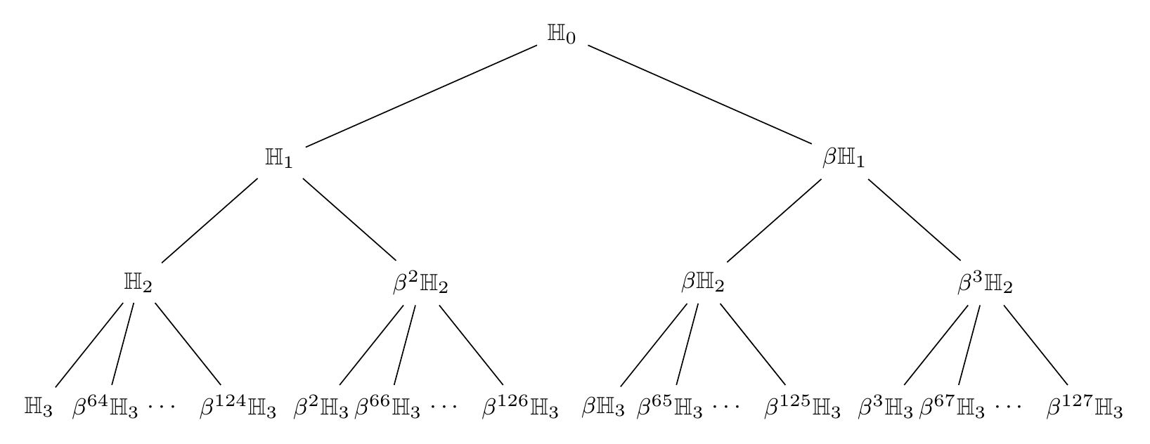
Figure 2 Tree of subgroups for BC code. Here, \beta is a generator of \mathbb{H}_0.
The exact algorithm using FFT is presented next. Let us use {\bf u} \in \mathbb{F}_q^{64 \times 128} to denote blob 0. We use {\bf u}[\textsf{start}\text{-}\textsf{end}] to denote the data at the cells \text{Cell}(0,\textsf{start}) to \text{Cell}(0,\textsf{end}). Let us define four (D\times \omega) = (64 \times 32) blob data arrays in their vectorized form, i.e., as 2048 long vectors:
The extended blob is denoted by {\bf \hat{x}} \in \mathbb{F}_q^{64 \times 256} and we have
again in vectorized form. We use || to concatenate two vectors one after another to form a longer vector. The algorithm is given below.
For i=0,1,2,3, execute:
-
If i is even, set \mathbb{G} = \beta \mathbb{H}_2, j=2i, \ell = (2i+2)\bmod 8.
-
If i is odd, set \mathbb{G} = \beta^3 \mathbb{H}_2, j=(2i+2)\bmod 8, \ell = 2i.
-
Set ((\hat{\mathbf{x}}_j \| \hat{\mathbf{x}}_\ell)(\alpha), \alpha \in \mathbb{H}_1) = \mathbf{u}_j \| \mathbf{u}_\ell.
-
Compute \mathbf{x}_j \| \mathbf{x}_\ell = \mathrm{IFFT}_{\mathbb{H}_1}(\hat{\mathbf{x}}_j \| \hat{\mathbf{x}}_\ell).
-
Compute \hat{\mathbf{x}}_{2i+1} = \mathrm{FFT}_{\beta\mathbb{H}_1}(\mathbf{x}_j \| \mathbf{x}_\ell, \mathbb{G}).
Entries of \hat{\mathbf{x}}_{2i+1} occupy cells respecting the coset assignment to each cell.
The above BC encoder requires four IFFT computations over \mathbb{H}_1 and four restricted FFT computations over \beta\mathbb{H}_1 restricted to a coset of \mathbb{H}_2. It may be noted again that |\mathbb{H}_1|=k_0D and |\mathbb{H}_2|=k_0D/2. By restricted FFT, we mean the computation of FFT over a group (coset) restricted to a subset of values belonging to subgroup (subcoset). An efficient way to compute restricted FFT/IFFT is provided in SVF2026.
Reconstruction algorithm
An efficient reconstruction algorithm is described in SVF2026.
KZG Commitments for Stacked BC Code
In every column of the stacked BC code, we have evaluations over a subgroup or a coset of a subgroup. Therefore, the KZG multiproof available for 1D RS code WZ2024 is applicable here as well. It is sufficient to have KZG commitments for each local RS code with a blocklength much smaller than the blocklength of the entire BC code. In this way, we reduce the complexity of KZG related computations.
Comparison With 1D and 2D RS Codes
Consider a BC code with parameters \mu, \omega and \rho. We fix the overlap factor \lambda=2 throughout the discussion. Recall that \mu represents the number of local codes, \rho D represents the number of redundant symbols in every local code, and \omega D represents the number of symbols at which two adjacent local codes intersect. The rate R, stopping rate S and local code size L of a BC code are given by:
The tradeoff between S and R for a BC code with different values of \mu is shown in Figure 3. The plots also contain the tradeoff for 1D and 2D RS codes. Thus the BC code achieves a region between 1D and 2D RS codes.
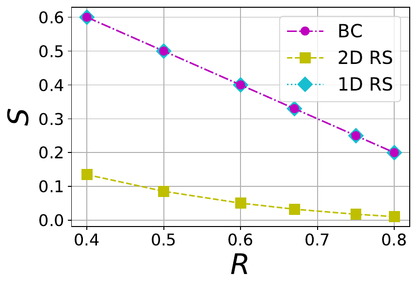
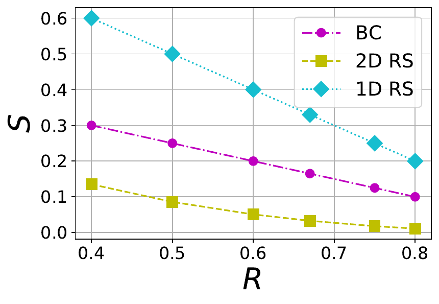
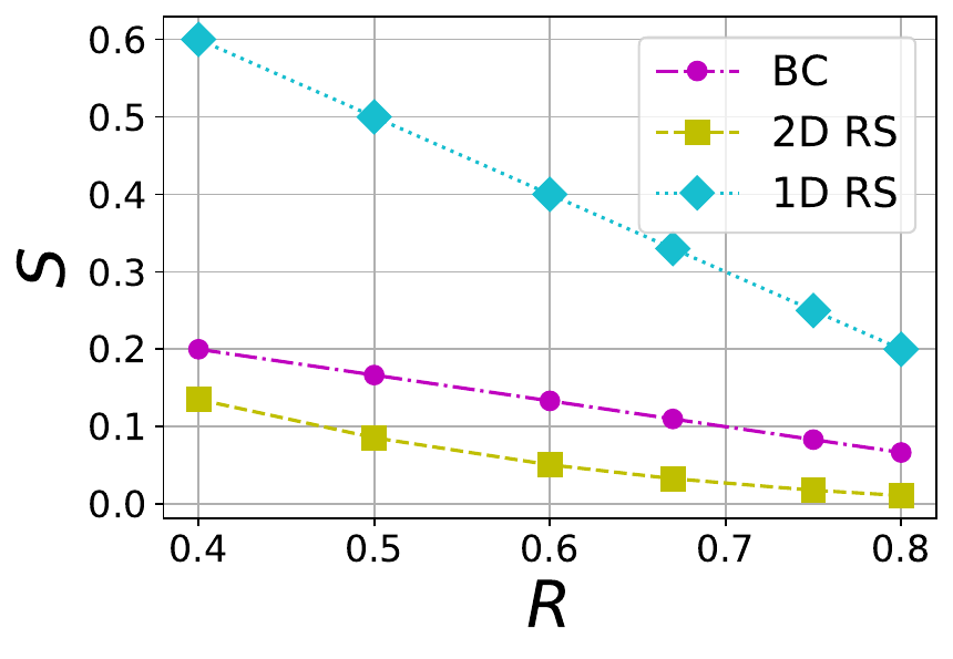
Figure 3 The tradeoff between stopping rate (S) and rate (R) in 1D RS, 2D RS and BC codes with different values of \mu=2,4,6 (left to right)
The absolute maximum number E of missing symbols that can be reconstructed within an extended blob is given by
where nD is the total number of symbols present in an extended blob and S is the stopping rate. We consider three different blob sizes 1 MB, 8 MB and 32 MB, and each of them maps to a certain number of finite field symbols kD within a blob. The mapping depends on the choice of finite field \mathbb{F}_q because a symbol in \mathbb{F}_q is represented using \lceil\log_2(q)\rceil bits. For example, an 1 MB blob is associated with 2^{15} finite field symbols when the the finite field is chosen to be the one linked to \texttt{bls12-381} with \lceil\log_2(q)\rceil = 32\times 2^8 = 32 bytes. For various file sizes, we plot E versus R in Figures 4 and 5. In Figure 4, a BC code with \mu=4 is compared against 1D and 2D RS codes whereas in Figure 5, a BC code with \mu=6 is chosen for comparison. It is no surprise that BC code is inferior to 1D RS code because 1D RS code is optimal with respect to E for a given rate. What is interesting is that BC codes with both \mu=4 and \mu=6 perform significantly better than the corresponding 2D RS code for the same file size and rate.
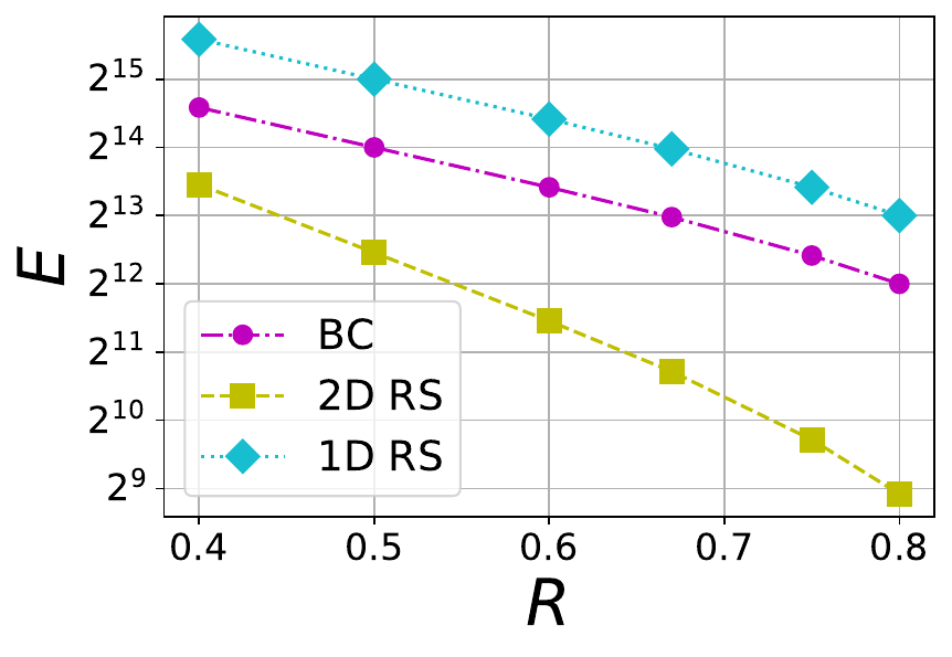
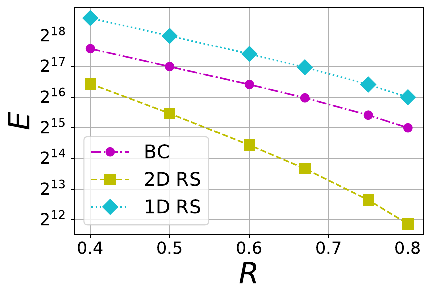
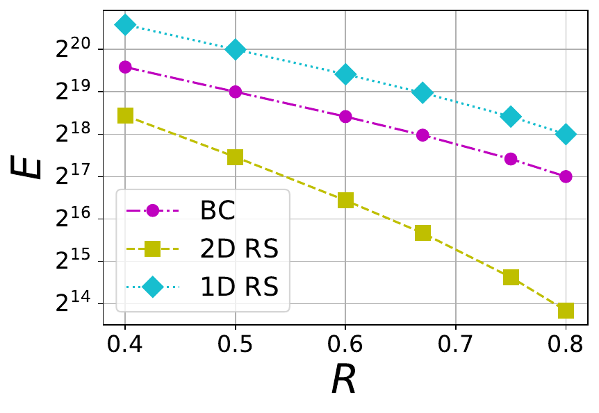
Figure 4 The tradeoff between tolerable number of erasures (E) and rate (R) in 1D RS, 2D RS and BC codes with \mu=4 and different file sizes F=1 MB, 8 MB and 32 MB (from left to right).
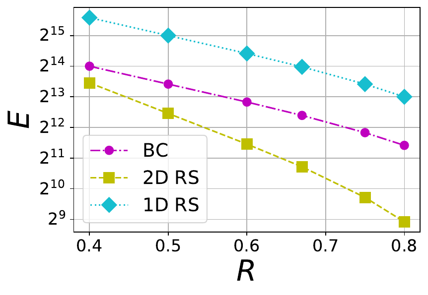
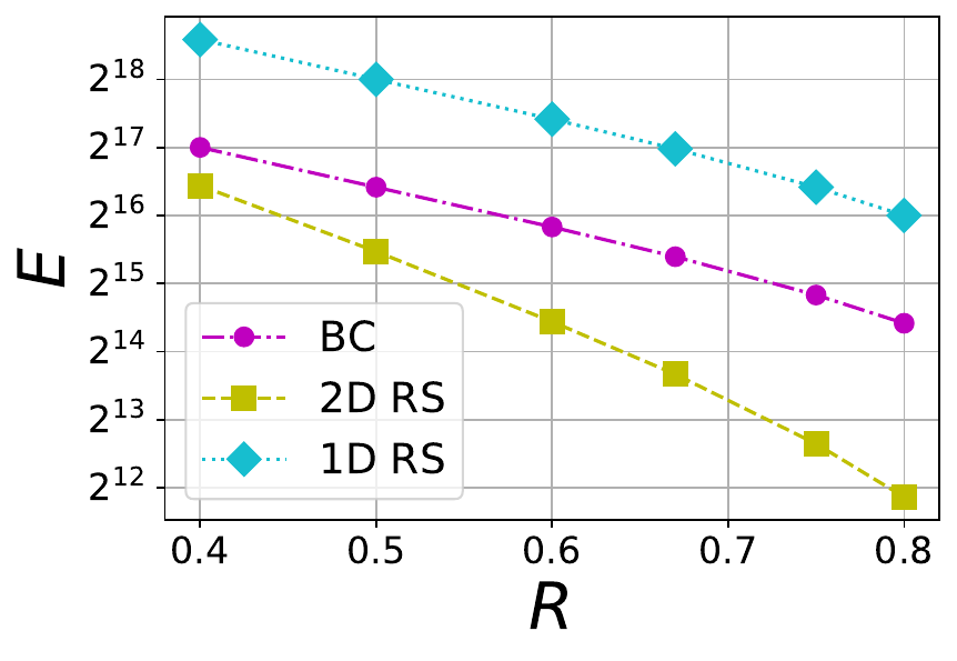
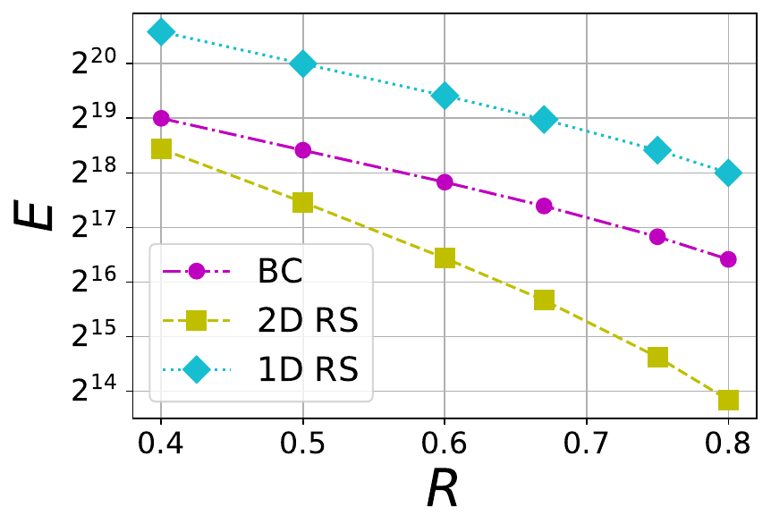
Figure 5 The tradeoff between tolerable number of erasures (E) and rate (R) in 1D RS, 2D RS and BC codes with \mu=6 and different file sizes F=1 MB, 8 MB and 32 MB (from left to right).
In Figure 6, the size of local codes within BC, 1DRS and 2DRS codes are compared. Since an 1D RS code does not contain any local code, the entire code is considered as its local code. It may be observed that 2D RS codes are significantly better than the BC code in absolute size of local code. In summary, a BC code gives a significant advantage in increasing the number of tolerable erasures with regard to the 2D RS code. However, the local code size of a BC code is very large compared to 2D RS code. In any case, the BC code offers a regime of operation different from that of both 1DRS and 2DRS codes, and opens up the possibility of designing codes operating on the intermediate regime between 1D and 2D RS codes.
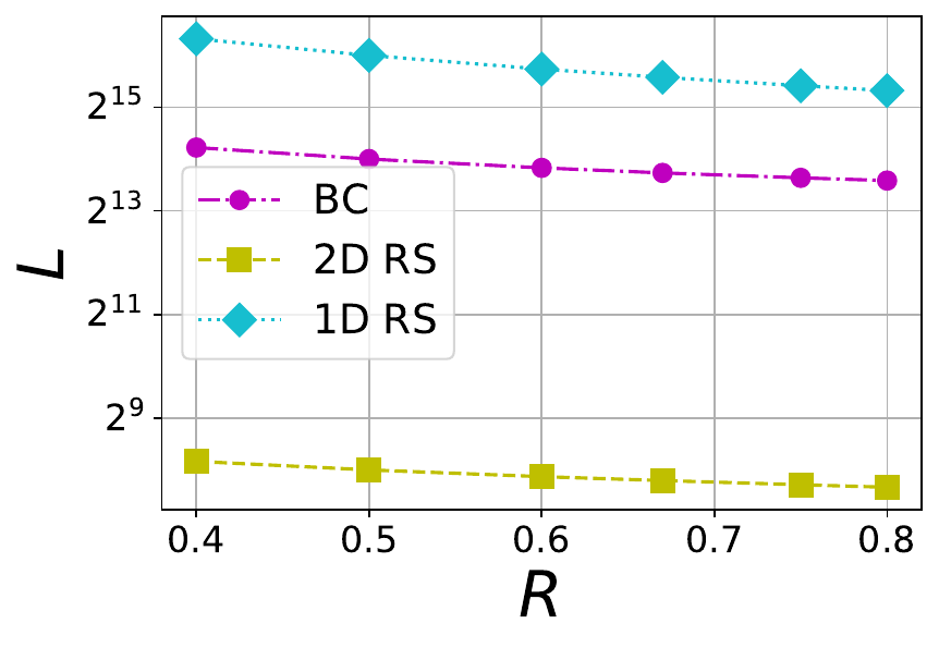
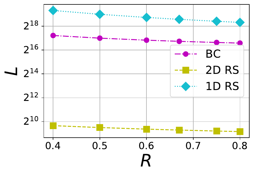
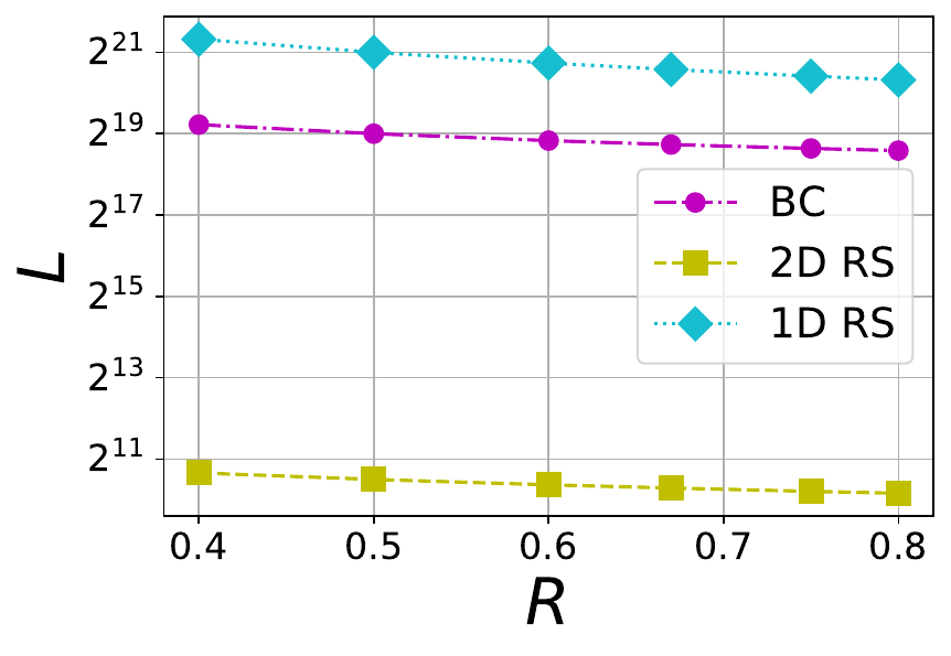
Figure 6 The tradeoff between local code size (L) and rate (R) in 1D RS, 2D RS and BC codes with \mu=6 and different file sizes F=1 MB, 8 MB and 32 MB (from left to right). For 1D RS there is no local code, so we take L=nD
References
[SVD2025] Theory of Block Circulant Codes
[SVF2026] Block Circulant Codes for PeerDAS
[WZ2024] A Documentation of Ethereum’s PeerDAS