This essay is authored by the MEV-X research team together with academic collaborators from HSE University.
Abstract
DeFi markets are efficient at the macro scale but constantly dislocated at the micro level: almost every swap moves a pool away from the market price and opens an arbitrage opportunity. We measure the dislocation value — the pool’s fee revenue plus the arbitrageur’s profit — and how it is split, as a function of the fee the pool charges on the arbitrage.
We find that an AMM maximizes the dislocation value by charging a zero fee on arbitrage. On today’s markets this does not happen, because the pool and the arbitrageur are two independent participants, each maximizing its own profit. As a result, constant-product AMMs (x \cdot y = k) run into a theoretical ceiling of 50% of the dislocation value, and on a live market they do not reach even that.
The solution is to merge the roles: using AMM hooks, the pool executes an atomic, internal arbitrage after each swap, capturing value that would otherwise be left unrealized or extracted by external searchers.
Introduction
Suppose that after some arbitrary event the market is in an inefficient state, an arbitrage opportunity exists, and there is an arbitrageur who will execute it as efficiently as possible.
A dislocation has at most two claimants: the arbitrageur keeps a profit, and the pool keeps a fee. We call their sum the dislocation value: everything the market inefficiency releases, no matter who ends up holding it.
The pool controls one parameter, the fee on arbitrage, and it determines two things:
- how large the dislocation value is;
- what share of it the pool keeps as fees.
The rest of this essay measures both effects. Table 1 collects the terms used throughout.
| Term | Meaning |
|---|---|
| Pool A | the volatile pool, whose price a retail swap knocks off the market price |
| Pool B | the reference pool, which holds the initial market price. The arbitrageur executes the arbitrage against this pool |
| \delta | the price dislocation: the price spread between the volatile pool and the reference pool, in percent, measured against the reference price, \delta = (P_A - P_B)/P_B |
| f | the fee on arbitrage: the fee the AMM charges on the arbitrage operation. This is not the retail fee, which stays positive throughout |
| Arbitrage revenue | the profit the arbitrageur keeps after executing the optimally sized arbitrage |
| Fee revenue | the fee the pool collects on the arbitrage swap |
| Dislocation value | arbitrage revenue plus fee revenue |
| Value left unrealized | dislocation value at f = 0 minus dislocation value at f |
The simulation: a numerical estimate of dislocation value
We estimated the behavior of the dislocation value numerically, by simulating the arbitrage across a range of fees on arbitrage. The result is clear: at a zero fee on arbitrage, the dislocation yields its maximum value. At any positive fee, part of that value disappears — not transferred to anyone, but left unrealized. Below we present the numerical details.
Results of the simulation
At a zero fee on arbitrage the dislocation yields its maximum, $24.75, and every cent of it goes to the arbitrageur. At 0.9901% and above, the fee exceeds what the arbitrageur can recover from the dislocation: the arbitrage never happens, the pool earns nothing, and the mispricing simply stands. Figure 1 shows the whole sweep.
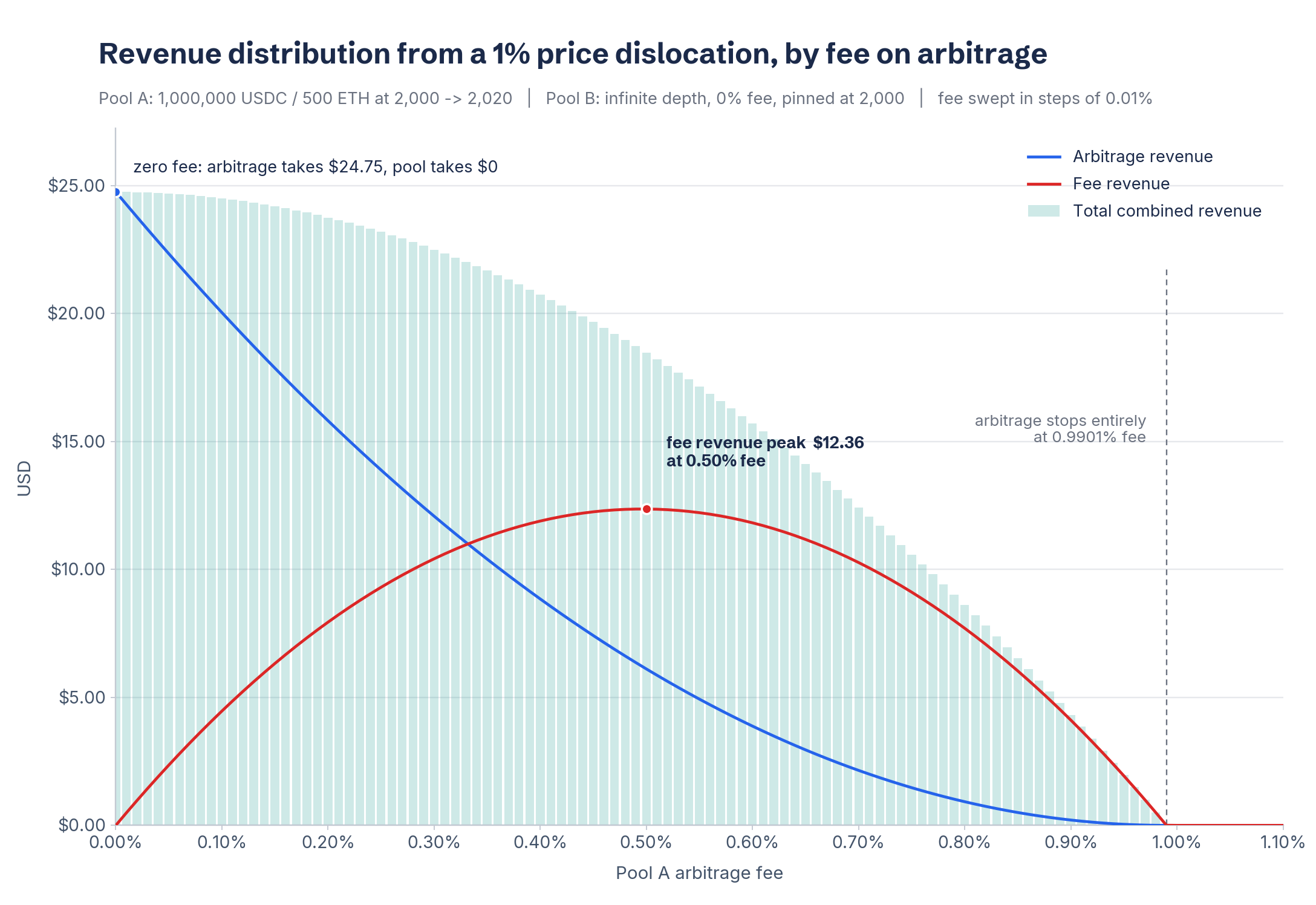
Figure 1: Arbitrage revenue, fee revenue and dislocation value as a function of the fee on arbitrage f, for a 1% dislocation (\delta = 1\%) in a 1,000,000 USDC / 500 ETH constant-product pool against an infinitely deep, fee-free reference pool. The bars are the dislocation value; the two lines are the shares the arbitrageur and the pool keep out of it. f swept in 0.01% steps.
Three things follow:
-
The maximum dislocation value is reached at a zero fee on arbitrage. Every increase in f lowers it, monotonically. At the fee that maximizes fee revenue the total has already fallen to $18.47, which is 74.62% of the maximum. The missing 25.38% is not transferred to anyone. It is left unrealized in the pool as an unclosed dislocation, because the arbitrage stops before the pool has been re-priced.
-
The maximum fee revenue is reached at a fee of about \delta/2. In our case the optimal fee is 0.50%, and it extracts $12.36, or 49.94% of the maximum dislocation value.
-
A constant fee is optimal for exactly one dislocation size and wrong for every other. At the conventional 0.30% the pool takes $10.42, which is 42.08% of the maximum, while the arbitrageur still realizes $12.08. Against a dislocation of 0.3%, that same 0.30% fee sits above the point where arbitrage stops, so the pool earns nothing at all.
Robustness across markets and AMM formulas
We repeated the sweep across nine markets (Figure 2): pool B at 0.5x, 1x and 10x the liquidity of pool A, and \delta at 0.3%, 1% and 10%. The shape is universal — only the dollar scale changes. The fee-revenue peak varies from 49.9–50.0% of the maximum at a 0.3% dislocation to 47.1–49.1% at a 10% one, approaching 50% as the dislocation gets small.
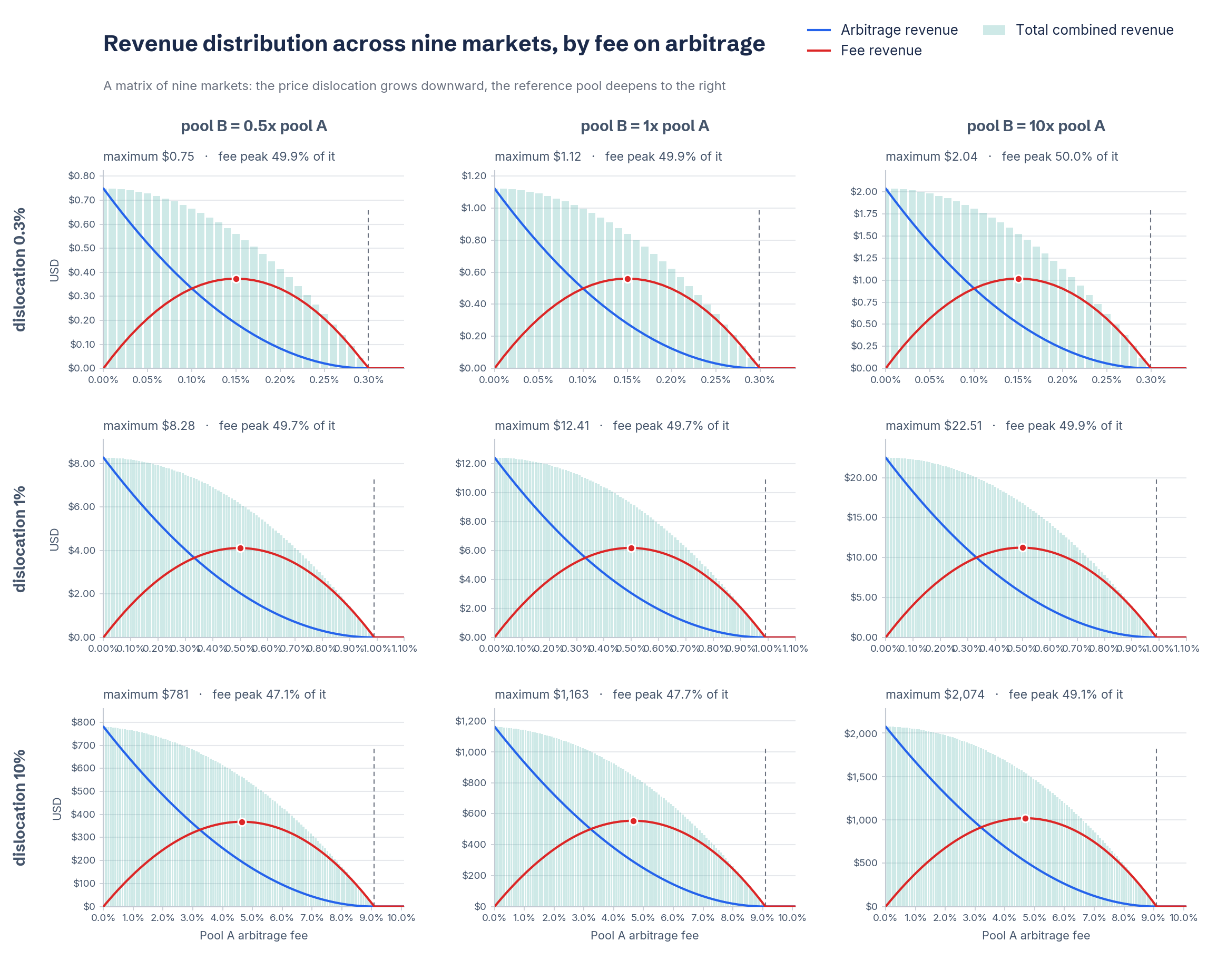
Figure 2: The same measurement repeated across a matrix of nine markets. Each panel keeps its own dollar scale, so what the matrix compares is shape, not size.
The same holds under other AMM formulas. We ran the same sweep on six architectures: Uniswap V2, Uniswap V3 concentrated liquidity, Balancer weighted, Curve CryptoSwap, Trader Joe Liquidity Book and DODO PMM. The zero-fee optimum holds on every one of them, at every dislocation size we tested. The maximum fee revenue, however, varies with the AMM formula, and each type of AMM needs its own treatment.
Generalization: two propositions
Neither property is a special case of one pool. Both are fundamental properties of how the dislocation value of an AMM behaves on an inefficient market. We state them as two propositions.
Proposition 1 (Zero-Fee Joint Optimum). Charging a fee on arbitrage never increases the dislocation value. Therefore, the maximum dislocation value is always achieved at zero fee.
Scope. Proposition 1 holds for any AMM whose marginal price is non-decreasing and integrable: continuous curves, piecewise smooth curves such as concentrated liquidity, and discrete step functions such as a liquidity book. It also holds when the reference pool has finite depth. Appendix A states the axioms and proves both cases (Theorems A.1 and A.4).
Proposition 2 (The 50% Ceiling for Constant Product AMMs). For a constant-product AMM where the marginal price is p(x) = k/x^2, and a small dislocation, a liquidity provider who tunes the fee on arbitrage to maximize its own fee revenue captures approximately 50% of the zero-fee maximum.
Appendix A proves it as Theorem A.2. Unlike Proposition 1, this one is not universal. For a general AMM whose price impact curve has non-linear local curvature, the peak fee revenue under an optimally tuned fee is not necessarily 50% of the maximum: the exact ceiling depends on the local elasticity of the price impact curve. The direction of the argument never changes, because a positive fee never increases the dislocation value.
AMM liquidity provider and arbitrageur: from adversaries to convergence
Here lies the paradox: the pool maximizes dislocation value at a zero fee, but a zero fee means gifting the profit to an external searcher. The pool has no reason to quote a zero fee to an outsider who will keep the proceeds. The arbitrageur has no reason to hand its profit to the pool. The positions of both players are rational, and each of them seeks to maximize its own profit.
As a result of these independent actions, part of the dislocation value is left unrealized. On a live market the price dislocation is often smaller than the fee, or only slightly larger, and as a result what is left unrealized is not 25% but most of the potential dislocation value.
Moreover, an AMM often has no way at all to distinguish an arbitrage swap from an ordinary retail swap, cannot calculate the price dislocation, and cannot set an optimal fee on such an operation.
The solution is to merge the roles of the AMM and the arbitrageur. AMM hooks made this technically possible. They allow the rebalancing arbitrage to execute atomically, in the same transaction as the retail swap, through an afterSwap hook. The pool grants the exclusive right to rebalance itself to its own logic. No external searcher can capture the rebalance, because there is no window between the user’s swap and the pool’s own reaction.
Two conditions make this work:
-
The zero fee applies only to the pool-initiated arbitrage operation. Retail traders keep paying a normal fee, and that fee is what pays the pool for providing liquidity.
-
Execution is internal and atomic. There is no competition with other searchers for the right to execute, no priority fee auction and no MEV leakage to a builder.
Arbitrage is not a standalone operation. It is a reaction to the user’s swap, opposite in direction, and it drives the pool back toward the state it started in. How far back depends on the depth of the reference pool and on the fee: against a deep reference pool at a zero fee the pool returns almost exactly to its starting composition and price, while a shallower one or a positive fee leaves part of the divergence standing. So internalizing the rebalance does not only add revenue, it also undoes part of the divergence that the user’s swap created.
Conclusions
-
The maximum dislocation value available from a market inefficiency is the value of arbitraging it at a zero fee. Every fee schedule is a deduction from that number.
-
For the constant-product curve, and any curve whose price impact is locally linear, the quadratic f(\delta - f) law caps fee revenue at approximately 50% of the maximum when the dislocation is small, with the remainder split between the arbitrageur and value left unrealized.
-
Maximizing the dislocation value of an AMM on an inefficient market runs through the convergence of the liquidity provider and arbitrageur roles via atomic execution. MEV-X Homelander implements this solution using
afterSwaphooks to internalize arbitrage revenue for liquidity providers.
The full article, including the theorem proofs, is available here.