Circulating Supply Equilibrium for Ethereum and Minimum Viable Issuance during the Proof-of-Stake Era

Edit: The updating mechanics became corrupted in the old post so it was suggested to me to repost the text. This new version is significantly revised. In a conversation with Justin Drake he raised an interesting question. What happens to the equilibrium if the starting conditions are 2^{20} validators and b = 0.05, i.e. if the conditions are set such that even at 100 % staking, the yearly issuance cannot exceed the yearly burn? This was not accounted for and is a special case of the model for how the deposit ratio and burn rate relate to the circulating supply from a later section, but setting d = 1. I have moved the equation earlier in the text to cover this case. Furthermore I have extended the modeling (new Section 4 and 5), edited the text for content and added figures to illustrate the current policy. Modeling and visualization of the circulating supply equilibrium under current policy is now the main focus of the text.


Hello. I’m a researcher from another field (mainly machine learning) and find blockchain tech very interesting. I have been following Ethereum for a while and appreciate the ethos of openness. The effects of a deflationary Ethereum, and the potential equilibrium for the circulating supply, seem to me like relevant topics to explore. Feel free to correct things I may have gotten wrong.


Abstract

This text explores potential equilibria for the circulating supply of Ethereum. The equality where yearly issuance equals yearly burn is used to create an equation for how the equilibrium depends on burn rate and deposit size. Other relationships are also presented, such as how staking yield relates to deposit size, the impact of potential active validator caps, as well as how both the equilibrium and the deposit ratio can be derived from yield and burn rate. The equations are then extended to account for assumptions for how the burn rate will be constrained by increasing deposit sizes and how the demand for yield changes across deposit ratio. The relationships are plotted across reasonable assumptions concerning variable values. A base case of around 2.5 % burn rate and stabilized demand for staking at 3 % yield are positioned within the plots; it gives equilibria between 27.3-49.5 million ETH depending on model. The text concludes by discussing if a minimum viable issuance policy, sustained by an adaptive base reward factor, could be beneficial for Ethereum. Such a policy could lead to perpetual deflation.

1. Introduction

With the introduction of EIP-1559, a deflationary mechanism has been added to Ethereum, burning base fees. This mechanism counteracts the inflation from ETH issued for securing the network. From a “monetary policy” perspective, it could be good to estimate the equilibrium for the circulating supply under current circumstances, and to make some projections for different equilibria under various assumptions (see the active validator cap proposal, and other discussions that are connected to, or implicitly depend on, estimates of the future circulating supply). The purpose of the text is to provide insights into how different variables in the ecosystem relate to each other and how they affect the equilibrium of the circulating supply. Independently, the larger question of minimum viable issuance under proof of stake is also discussed towards the end of the text. Here input from the community would be needed to highlight potential drawbacks and benefits of such a policy.

Section 2 briefly reviews the current burn rate and proof-of-stake issuance. In Section 3, the basic equation for the circulating supply equilibrium is stipulated and then extended to account for corner cases and active validator caps. The connection between staking yield and deposit size is also examined. Section 4 introduces a constrained burn-rate model that expects a reduced burn rate with an increase in staking. Section 5 investigates the relationship between burn rate, yield, and deposit ratio at the equilibrium. An adaptive yield demand curve is also introduced to account for how the demand for staking yield may vary across deposit ratio. This section also relates the deposit ratio to minimum viable issuance in the proof-of-stake era, something that is further examined in Section 6 where a variable base reward factor is shown to facilitate such an issuance policy. This could create perpetual deflation. Some benefits and drawbacks of such a policy are offered and conclusions are provided in Section 7.

2. Current statistics

Since its inception, EIP-1559 has burned close to 8 000 ETH/day. This corresponds to a yearly burn B of around 2.9 million ETH. Given the current circulating supply S \approx 117.4 million ETH (as of September 2021), the burn rate is given as b = B/S \approx 0.025. Thus, around 2.5 % of the circulating supply is burned each year at the current burn rate.

The current deposit size D for the staking contract is around 7.5 million ETH. The yearly issuance I of ether to validators under proof of stake can be computed from the deposit size and the base reward factor F as

I = cF \sqrt{D}

where c is a constant c \approx 2.6 derived from the number of epochs in each year and compensating for the fact that the protocol denominates ether in gwei. The base reward factor F is controlled by the developers and is set to 64. Since it determines issuance, and thus how high rewards are for staking, it can be used to control staking demand in Ethereum, as discussed in Section 6. Inserting these numbers into the equation gives a yearly issuance of around 455 000 ETH.

3. Equilibrium under current policy and with an active validator cap

3.1 Equilibrium as a function of deposit size and burn rate

The yearly burned ether B can be modeled as a burn rate b of the circulating supply S,

B = bS,

The equilibrium when I = B gives

cF \sqrt{D} = bS,

which means that the circulating supply at the equilibrium will be

S = \frac{cF \sqrt{D}}{b}.

3.2 Equilibrium with burn rate higher than issuance at 100 % staking

What happens if the initial conditions are set such that even at 100 % staking, the yearly issuance does not exceed the yearly burn? This example is somewhat academic since it is hard to envision a lively transacting chain at close to 100 % staking (as further discussed in the following sections). But it should be modeled for completeness, and it also points to a need for exploring alternative models of the burn rate, which is done in Section 4.

The remainder of this section resolves the case when 100 % staking issuance is lower than the burn. This happens when

bD > cF \sqrt{D},

i.e., when D = S and the yearly burn B = bD, specified at a deposit size corresponding to the circulating supply is bigger than the issuance I = cF \sqrt{D} at the same deposit size. To understand why S can be replaced by D in the equation, consider that D can never be larger than S, which means that bD can never be larger than bS. If the yearly burn bD is larger than issuance, then certainly so is the yearly burn specified as bS. The inequality can be simplified

b^2D^2 > c^2F^2D,

to derive the condition for when the burn rate is bigger than the issuance at 100 % staking,

D > \frac{c^2F^2}{b^2}.

The deposit size will in this case shrink each year until the equilibrium is achieved, which happens when

D = \frac{c^2F^2}{b^2},

which provides us with the equation for the ultimate circulating supply when the inequality is true

S = \frac{c^2F^2}{b^2}.

The equilibrium is in this case thus reached independently of the initial deposit size. Combining the findings, the complete equation is:

S = \left\{ \begin{array}{ c l } \frac{c^2F^2}{b^2} & \quad \textrm{if } D > \frac{c^2F^2}{b^2} \\ \frac{cF \sqrt{D}}{b} & \quad \textrm{otherwise} \end{array} \right..

3.3 Equilibrium relative to staking yield and burn rate

To produce a base case for a potential equilibrium using the proposed model, it is necessary to estimate variables b and D. Since a rather wide range of variable values is reasonable, the plots of this and the following sections show the equilibrium across wide ranges, so that the reader can draw their own conclusions. Still a specific “base case” can help. The current approximate burn rate of 0.025 can be used. To define a reasonable D it is instead best to first estimate the yield y around which staking demand and thereby the deposit size D will stabilize. The issuance can be described as I = yD as well as I = cF \sqrt{D}; the equality can be used to derive how D depends on yield:

yD = cF \sqrt{D},

y^2D^2 = c^2F^2D,

D = \frac{c^2F^2}{y^2}.

The yield at which staking demand stabilize could for example be set to 3 % in the base case. This would give a deposit size of

D = \frac{c^2F^2}{y^2} = \frac{2.6^2 \times 64^2}{0.03^2} \approx 30.7 million ETH.

Such a deposit size gives an equilibrium of

S = \frac{cF \sqrt{D}}{b} = \frac{2.6 \times 64 \sqrt{30.7 \times 10^6}}{0.025} \approx 36.9 million ETH.

The complete equation for how the equilibrium depends on burn rate and stabilized staking yield can also be derived. It is:

S = \frac{cF \sqrt{\frac{c^2F^2}{y^2}}}{b},

S = \frac{c^2F^2 }{yb}.

3.3.1 Introducing an active validator cap

If an active validator cap is applied and reached, the relationship between yield and deposit size changes, and the equilibrium also becomes independent of deposit size (note that with the constrained burn-rate model introduced in Section 4, this is no longer true, because that model assumes that increased staking will push down the burn rate). Setting the cap at L validators, the yearly issuance can be defined as cF \sqrt{32L}, and the deposit size at the equilibrium when the yield stabilizes can be derived directly from

yD = cF \sqrt{32L}

as

D = \frac{cF \sqrt{32L}}y.

At a 3 % yield, when setting the active validator cap to 2^{19} validators, the deposit size for the base case would be

D = \frac{2.6\times64\sqrt{32\times2^{19}}}{0.03} \approx 22.7 million ETH.

However, since issuance is fixed when the cap is reached, the equilibrium for the base case is derived independently of D as

S = \frac{cF \sqrt{32L}}{b} = \frac{2.6 \times 64 \sqrt{32 \times 2^{19}}}{0.025} \approx 27.3 million ETH.

3.4 Illustrating the equilibrium

Figure 1 shows how the equilibrium varies with deposit size, staking yield (with or without an active validator cap) and burn rate. The figure is generated by using the equations developed in this section and the base cases are indicated with circles. Note that the circulating supply is computed without an applied active validator cap, which would bound the circulating supply S above it in the figure, independent of the deposit size.

Figure 1. The circulating supply Equilibrium for Ethereum under current policy, plotted against the deposit size D (left y-axis), yield (right y-axis) and burn rate b = B/S (x-axis). Dashed lines indicate potential active validator caps which, if applied, would bound the circulating supply S above the line. They are assumed to not be applied in this figure, except for beige annotations. Among these, the yield with an active cap (beige) is positioned relative to D but the corresponding equilibrium for S can be found at the actual cap (indicated by dashed beige arrow). Thin dotted lines indicate the circulating supply at 20, 40, and 80 million ETH (note that S is log-scaled). Plotted in white is the limit at which burned ether equals issuance from 100 % staking. This line is unlikely to be reached since the burn rate can be expected to fall at very high staking ratios. The circled base cases indicate circulating supply equilibria for a 2.5 % burn rate and 3 % yield with (beige) or without (red) an active validator cap at 2^{19} validators. Vector graphics for the figure: Equilibrium under Current Policy.pdf (125.3 KB)

4. Equilibrium under current policy with a constrained burn rate

4.1 Without an active validator cap

As mentioned in the previous Section 3, there is reason to consider a modification of the definition of the burn rate. When the deposit ratio is high, the burn rate as a proportion of the total circulating supply can be expected to fall. In this scenario, holders prefer to stake their ether over using it transacting on-chain. To account for this, in order to better model how present burn rates translate to future burn rates, the constrained burn rate b' can instead be defined as

b' = \frac{B}{S-aD},

with reduced burning of staked ether. The more ether that is staked, the less is burned. The variable a determines the proportion of staked ether to be unaccounted for when computing the constrained burn rate. The circulating supply equilibrium under a constrained burn rate is given by inserting the redefined yearly burn b'(S-aD) into the equality of yearly issuance and burn:

b'(S-aD) = cF \sqrt{D},

S = \frac{cF \sqrt{D}}{b'} + aD.

The circulating supply when the yearly burn is higher than yearly issuance at full staking can be determined in a similar way as in Section 3.2. The inequality for higher burn than issuance at S = D is

b'(D-aD) > cF\sqrt{D},

which can be resolved to

D^2(1-a)^2 > \frac{c^2F^2D}{b'^2},

D > \frac{c^2F^2}{b'^2(1-a)^2}.

The deposit size will in this case shrink each year until the equilibrium when

D = \frac{c^2F^2}{b'^2(1-a)^2},

and thereby

S = \frac{c^2F^2}{b'^2(1-a)^2}.

The equation for the circulating supply with a constrained burn rate model can thus be derived as

S = \left\{ \begin{array}{ c l } \frac{c^2F^2}{b'^2(1-a)^2} & \quad \textrm{if } a \neq 1 \textrm{ and } D > \frac{c^2F^2}{b'^2(1-a)^2} \\ \frac{cF \sqrt{D}}{b'} + aD & \quad \textrm{otherwise} \end{array} \right..

If a is set to 1, only the non-staked ether is included when computing the burn rate. However, such a strong assumption is likely incorrect. At very high deposit ratios, participants in the ecosystem are likely using derivatives of staked ether (e.g., stETH) for many use cases, converting to ETH specifically for paying transaction fees. So while a = 0 (the definition used in Section 3) may overestimate the burn when projecting current burn rates to scenarios with a higher deposit ratio, a = 1 (only non-staked ether is included when modeling burn rate) may instead underestimate the burn. Setting a = 0.5 seems like a reasonable compromise at this point.

It is now possible to compute the equilibrium for the base case. The constrained burn rate is b' = B/(S-aD) \approx 0.027 when using current statistics. Stabilized staking demand at 3 % yield gives a deposit size of 30.7 million ETH, as computed in Section 3.3. The equilibrium is thus

S = \frac{cF \sqrt{D}}{b'} + aD = \frac{2.6 \times 64 \sqrt{30.7 \times 10^6}}{0.027} + 0.5 \times 30.7 \times 10^6 \approx 49.5 million ETH.

Figure 2 shows how the circulating supply equilibrium varies with D and b', using a = 0.5. Note that the condition where the burn rate equals 100 % staking (white line in Figure 1) is outside of the boundaries of this figure. With a constrained burn rate of 0.04 (the right edge of the x-axis), the condition is only met at

D = \frac{c^2F^2}{b'^2(1-a)^2} = \frac{2.6^2 \times 64^2}{0.04^2(1-0.5)^2} \approx 69.2 million ETH,

or conversely with a 40 million deposit size, at a constrained burn rate of

b' = \frac{cF}{\sqrt{D}(1-a)} = \frac{2.6 \times 64}{\sqrt{40 \times 10^6}(1-0.5)} \approx 0.053.

Figure 2. The circulating supply Equilibrium for Ethereum under current policy using a constrained burn-rate model, plotted against the deposit size D (left y-axis), staking yield (red, right y-axis) and constrained burn rate b’ (x-axis). Dashed lines indicate potential active validator caps which are not applied. Thin dotted lines indicate the circulating supply at 20, 40, and 80 million ETH (note that S is log-scaled in the figure). The red circle indicates the base case with b’ = 0.027 and stabilized demand for staking at 3 % yield, which gives an equilibrium of 49.5 million ETH when using the constrained burn-rate model. Vector graphics for the figure: Equilibrium - constrained burn rate.pdf (148.0 KB)

4.2 With an active validator cap

When using the constrained definition of the burn rate b' under a policy with an active validator cap, inactive validators will serve to raise the equilibrium for the circulating supply. The fact that ether locked up by validators cannot be used for transacting is assumed to reduce the rate at which ether is burned. When the number of validators is higher than the active validator cap L, the point where yearly issuance equals yearly burn is

b'(S-aD) = cF \sqrt{32L},

which can be resolved into the equation for the equilibrium

S = \frac{cF \sqrt{32L}}{b'} + aD.

The circulating supply when the yearly burn is higher than yearly issuance at full staking once again needs to be determined. With an active validator cap, the inequality for higher burn than issuance at S = D is

b'(D-aD) > cF\sqrt{32L},

which can be resolved to

D(1-a) > \frac{cF\sqrt{32L}}{b'},

D > \frac{cF\sqrt{32L}}{b'(1-a)}.

The deposit size will in this case shrink each year until the equilibrium when

D = \frac{cF\sqrt{32L}}{b'(1-a)},

and thereby

S = \frac{cF\sqrt{32L}}{b'(1-a)}.

The conditional statement for the equilibrium when using an active validator cap is then

S = \left\{ \begin{array}{ c l } \frac{cF\sqrt{32L}}{b'(1-a)} & \quad \textrm{if } a \neq 1 \textrm{ and } D > \frac{cF\sqrt{32L}}{b'(1-a)}\\ \frac{cF \sqrt{D}}{b'} + aD & \quad \textrm{elseif } D < 32L \\ \frac{cF \sqrt{32L}}{b'} + aD & \quad \textrm{otherwise} \end{array} \right..

The deposit size at 3 % staking yield and an active validator cap is the same as established in Section 3.3.1, 22.7 million ETH. Using b' = 0.027, the circulating supply at the equilibrium is

S = \frac{2.6 \times 64 \sqrt{32 \times 2^{19}}}{0.027} + 0.5 \times 2.27 \times 10^7 \approx 36.6 million ETH.

Figure 3 shows how the circulating supply varies with the deposit size and the constrained burn rate b’ when the active validator cap is applied at 2^{19} validators. The computed equilibrium of 36.6 million ETH is indicated by a beige circle. The plot has been extended to D = 45 million ETH so that the dotted line indicating 40 million ETH stretches across all three conditions of the equation for the circulating supply.

Figure 3. The circulating supply Equilibrium S for Ethereum with an active validator cap at 2^{19} validators (black horizontal line) using a constrained burn-rate model, plotted against the deposit size D (left y-axis), staking yield (beige, right y-axis) and constrained burn rate b’ (x-axis). Thin dotted lines indicate the circulating supply at 20, 40, and 80 million ETH (note that S is log-scaled in the figure). The beige circle indicates the base case with b’ = 0.027 and stabilized demand for staking at 3 % yield, which gives an equilibrium of 36.6 million ETH when using the constrained burn-rate model. Vector graphics for the figure: Equilibrium - constrained burn rate - 2^19 cap.pdf (149.6 KB)

5. Relationship between burn rate, stabilized yield, and deposit ratio

5.1 Deposit ratio for previous examples

It can be noted that the deposit ratio

d = \frac{D}{S}

is rather high at the equilibrium for the base cases; 0.83 for the basic burn-rate model in Section 3: 30.7/36.9 \approx 0.83, 22.7/27.3 \approx 0.83, and 0.62 for the constrained burn-rate model in Section 4: 30.7/49.5 \approx 0.62, 22.7/36.6 \approx 0.62.

5.2 Minimum viable issuance and deposit ratio

Ethereum has had a policy of minimum viable issuance during the proof-of-work era, stipulating that the issuance of new tokens should be high enough to secure the blockchain, but not higher. Under proof of stake, the deposit ratio will be an important factor determining the security of the chain. If the deposit ratio is too low, Ethereum becomes less secure. A previous proposal suggests a Simplified Active Validator Cap at 2^{19} validators and 16.8 million ETH, corresponding to d \approx 0.14 at the current circulating supply. The purpose of the cap is to increase “confidence that a given level of hardware will always be sufficient to validate the beacon chain,”. One interpretation is that such a deposit ratio should ensure sufficient security, according to Buterin. Further input about the minimum viable deposit ratio for long-term security would be welcome from the community.

Are there any consequences of letting the deposit ratio become very high, i.e., is there a “too high” when it comes to the deposit ratio? This text does not answer that question, but attempt to provide some insights regarding the relationship between proof-of-stake variables that can be used in a further discussion. With an increasing deposit ratio, it seems inevitable that economic activity will be reduced in favor of locking up ether for staking. This reduces the “velocity of money” and adds an inflationary pressure both due to increased issuance and decreased burn rate. Although stakers can be expected to be more aligned with the interests of the network than miners, it seems as if a number of stakeholders of Ethereum could benefit from retaining a minimum viable issuance policy also under proof of stake. A further discussion is offered in Section 6.

To fully examine the issuance policy under proof of stake, it is desirable to understand how the deposit ratio relates to the burn rate and the yield at which staking demand stabilizes. This is done in the remainder of this section.

5.3 Deposit ratio as a function of yield and burn rate

As indicated in Section 5.1, the deposit ratio at the equilibrium can be derived independently of any validator cap as a function of the yield at which staking demand stabilizes and the burn rate. With the basic burn-rate model, the equilibrium of yearly burn and issuance,

bS = yD,

can be simplified to

\frac{D}S = \frac{b}y,

d = \frac{b}y.

For the constrained burn-rate model, the equilibrium of yearly burn and issuance,

b'(S-aD) = yD,

can instead be simplified to

\frac{S}D-a = \frac{y}{b'},

\frac{1}d = \frac{y}{b'}+a,

d = \frac{1}{y/b'+a},

d = \frac{b'}{y +ab'}.

The difference between the basic and constrained burn-rate model is thus that the constrained model reduces the deposit ratio at the equilibrium by adding ab’ to the denominator.

5.3.1 Visualization

Figure 4 shows how the deposit ratio varies depending on burn rate and the yield y at which staking demand stabilizes. The top pane uses the basic burn-rate model from Section 3 and the bottom pane instead uses the constrained burn-rate model from Section 4, with a = 0.5. As previously noted, the deposit ratio at the equilibrium is the same for examples with and without an active validator cap; it is independent of any such cap.

The white rectangles cover the range between 1 % to 3.5 % for the burn rate and between 2 % to 3.5 % for the stabilized staking yield. The purpose is to highlight a range that seems reasonable, but it is not yet possible to predict that the variables will reside within these particular ranges. The deposit ratio of 0.14 discussed in the context of “minimum viable issuance” in Section 5.2 is shown with a yellow line. As evident, the line falls outside of the variable ranges that can reasonably be expected (granted with insufficient knowledge about these ranges at this time). For some combinations of y and b, the deposit ratio reaches 1. In a real-world scenario, it will never reach 1, because many tokens are lost forever, and staking demand and burn rate will fall once the deposit ratio becomes very high. The following Subsection 5.3.2 addresses this.

Figure 4. The deposit ratio at the equilibrium for the circulating supply of Ethereum, relative to burn rate and the yield at which staking demand stabilizes. The top pane shows the relationship for the basic burn-rate model described in Section 3, and the bottom pane uses the constrained burn-rate model described in Section 4. The white rectangle encloses “reasonable” variable values, y = 0.02-0.035, b = 0.01-0.035, that may need to be updated once staking has been further established. The yellow line indicates d = 0.14, which corresponds to 2^{19} validators and was discussed in Section 5.2 related to minimum viable issuance. Vector graphics for the figure: Deposit ratio relative to yield and burn rate.pdf (198.0 KB)

5.3.2 Letting demand for staking yield vary with deposit ratio

So far in this text, the demand for yield has been modeled as independent of the deposit ratio. Such a model assumes that if the demand for staking will stabilize at 3 %, then the “marginal staker” is ready to stake their ether if the yield is at or above 3 %, but will not stake otherwise. This makes it possible to use both deposit size and stabilizing yield on the left and right sides of the y-axis in the figures in Sections 3-4. For Figure 4 there is however no such need and it would be possible to allow this yield to depend on the deposit ratio, which is a more realistic model. Some participants in the eco-system are likely dead-set to stake their tokens whatever the yield, and some will be very reluctant or unable to do so even if the yield is very high. A model that assumes that the yield will stabilize at for example 3 % could therefore use an adaptive yield that plateaus at 3 % for deposit ratios between 0.1 and 0.7, but trends to 0 % at d = 0 and reaches double-digits when d approaches 1. This would allow the model to investigate the effect of various yields without creating unrealistic edge cases, such as the white area in the top right corners of both the top and bottom panes in Figure 4. Naturally, the deposit ratio will never reach 1, and could only trend towards 0 if the burn rate is close to 0.

The adaptive yield y’ which depends on the deposit ratio could for example be generated by multiplying the assumed yield with

1+\frac{5d-1}{2}^3.

Figure 5 shows how such a y’ depends on the deposit ratio when the yield is set to 3 %. As evident, the curve was designed to follow the description in the first paragraph of this subsection. Another variant would have been to rework the odds function \frac{d}{1-d} which may behave more realistically when d approaches 1. It is impossible at this time to know how the yield demands of the “marginal staker” vary with deposit ratio, but hopefully the proposed model is more accurate than assuming a flat yield demand.

Figure 5. An adaptive yield demand curve at y’ = 3 %, devised to model how demand for yield may vary across the deposit ratio. At low deposit ratios, the “marginal staker” can be expected to demand a lower yield for staking than at normal deposit ratios. At high deposit ratios, it is expected that a very high yield is needed to convince the “marginal staker” to stake their ether. The estimate is very uncertain, but likely better than assuming a flat yield demand. Vector graphics for the figure: Devised adaptive yield demand curve.pdf (49.5 KB)

Having devised an adaptive yield demand curve, it is now possible to revise the plots for how the deposit ratio varies across stabilizing yield and burn rate. Figure 6 shows the deposit ratio at the equilibrium relative to the adaptive yield y’ and burn rate. As evident, the edge case where the deposit ratio reaches 1 (white triangular area in Figure 5) has been resolved at these variable ranges.

Figure 6. The deposit ratio at the equilibrium for the circulating supply of Ethereum, relative to burn rate and the adaptive yield at which staking demand stabilizes. The adaptive yield demand curve shown in Figure 5 is applied to y’ and varies across d. The top pane shows the relationship for the basic burn-rate model described in Section 3, and the bottom pane uses the constrained burn-rate model described in Section 4. The white rectangle encloses “reasonable” variable values, y = 0.02-0.035, b = 0.01-0.035, that may need to be updated once staking has been further established. The yellow line indicates d = 0.14, which corresponds to 2^{19} validators and was discussed in Section 5.2 related to minimum viable issuance. Note that d for the two panes extends over a slightly different range but with the same color encoding. Vector graphics for the figure: Deposit ratio relative to adaptive yield and burn rate.pdf (168.9 KB)

6. Enforcing minimum viable issuance with a variable base reward factor

6.1 Overview

Previous sections have served to build an understanding of Ethereum’s monetary policy in the proof-of-stake era. If the burn rate is sustained, then issuance as a proportion of the circulating supply will rise and rise until it equals burned ether. This policy will lead to a circulating supply equilibrium where issuance equals burn rate. The circulating supply will however continue to vary also after this point in line with varying demand for staking yield and block space over the years. As mentioned in Section 5.2, the deposit ratio could end up above minimum viable issuance based on reasonable assumptions concerning future burn rates and staking yields. What would be the effect of instead keeping yields at minimum viable issuance levels, so that Ethereum may become perpetually deflationary? Such a policy could benefit many stakeholders in the Ethereum ecosystem, with a higher velocity of money, and passive value accrual also to people who are not staking their ether. Formulated a little differently:

If Ethereum attracts a higher deposit ratio than what is strictly needed for security, would it serve the ecosystem better to slowly reduce yields (e.g., adjust the base reward factor), equally rewarding all holders and participants in the ecosystem in the form of deflation?

How could such a policy be enforced? As illustrated in Sections 3-5, neither an active validator cap nor a permanent one-time reduction of the base reward factor would lead to perpetual deflation. Instead, a gradual reduction of the base reward factor in phase with a changing deposit ratio due to burned ether would be needed. Trying to beforehand specify a particular deflation rate to be maintained each year would hardly be feasible. Both the burn rate and stabilized yield can be expected to fluctuate also over longer time spans in response to changes in economic outlook, new use cases, and technological progress. Thus, a deflation rate that may seem sustainable at first could a few years later produce too low or too high (if this is deemed undesirable) deposit ratios. Therefore, it is not desirable to specify a constant factor at which the base reward factor would change each year. Instead, it could be continuously adapted to the deposit ratio, potentially factoring in ether that has not been moved for a very long time (more on this in Section 6.3.2).

6.2 Example

An example may help for understanding. This example does not account for what is technically feasible or not; it merely illustrates how to enforce minimum viable issuance. At a point where a perpetual deflation policy has stabilized, the yield y could for example be 0.03, the burn rate b, 0.02, and the deposit ratio d at the desired 0.14 of the circulating supply S. The inflation/deflation rate s is

s = dy-b = -0.0158,

which corresponds to a yearly reduction of the circulating supply by 1.58 %. The circulating supply is thus changed by a factor of 0.9842 in one year.

6.2.1 Current policy

Stepping forward one year, if the current policy is used, the following would happen:

  • D – Assuming a flat yield demand curve, the marginal staker still demands 3 % yield to stake. Section 3.3 derived the equation for how deposit size depends on yield in this case D = \frac{c^2F^2}{y^2}, which gives that the deposit size will stay fixed if the yield demand is fixed and the base reward factor F left unchanged.
  • d – The deposit ratio will change since the circulating supply has been reduced. Thus at year 1, d_1 = 0.14S_0/(0.9842S_0) = 0.1422

As evident, the deposit ratio rises. This would continue until d = \frac{b}y \approx 0.67 assuming a flat yield demand curve and basic burn-rate model. The reason is that the issued and burned ether at year 0 is not an equilibrium and there needs to be a continuous reduction of the base reward factor if the goal is to maintain a deposit ratio of 0.14.

6.2.2 Perpetual deflation

To retain minimum viable issuance, the base reward factor F would instead need to be adaptively adjusted to keep the deposit ratio at a desired level (in this example, 0.14). For the given values, this require reducing the deposit size: D_1 = 0.9842D_0. Ignoring fixed variables in D = \frac{c^2F^2}{y^2}, the required adjustment to the base reward factor would be

F_1 = \sqrt{0.9842 \times {F_0}^2} = 0.9921F_0.

Thus, the base reward factor would be reduced by the square root of the desired change to the deposit size. Expressed more generally: The deposit ratio can, in theory, be maintained with a yearly change of F by a factor of

\sqrt{1+s}.

Note that the computations in this section do not account for gradual changes of the variables.

6.3 Further discussion of monetary policy

The current monetary policy of Ethereum under proof of stake has gained wide acceptance. It is simple, easy to maintain, and will lead to an equilibrium. Therefore it may seem unnecessary to discuss variations of the established policy. This section does not however take a stand in favor of a perpetual deflationary policy. It is merely assuming that discussing and exploring the alternatives can be fruitful. EIP-1559 has introduced a deflationary pressure that may not have been anticipated when the original proof-of-stake monetary policy was established.

6.3.1 Money Lego

As discussed in Sections 5.2 and 6.1, high deposit ratios could potentially slow down economic activity. One aspect that influences the “velocity of money” for Ethereum going forward is therefore the degree to which liquid staking derivatives, e.g., rETH, can be used as a substitute in economic activity. In such a scenario, participants in the eco-system can use derivatives in their daily activities, converting to ether only for paying transaction fees or for dealing with parties that only accept ether. It seems plausible that in a scenario where perpetual deflation is enforced, participants would be less likely to resort to derivatives since deflation (and subsequent token price appreciation) will capture the majority of the rewards from token burns.

Staking derivatives will add an extra layer to an anticipated “Money Lego” of Ethereum. Such arrangements may pose risks, not to the proof-of-stake consensus but to an ecosystem of DApps relying on these derivatives. The day before the launch of Rocket Pool an exploit was discovered, despite the protocol going through serious auditing beforehand. What would happen if participants are incentivized to interact within the Ethereum ecosystem using staking derivatives at the bottom layer, these permeate the ecosystem, and there is an exploit?

6.3.2 Long-term effect of deflation

A long-term effect of a deflationary Ethereum is that as the circulating supply shrinks, the proportion of lost ether in relation to the ether that still can be moved will rise. Importantly, this proportion will be unknown. Therefore, at the very long time frame, determining minimum viable issuance may become harder, or such attempts even undesirable. Another aspect when rewards are accrued mainly through deflation is that this will reward holders that are very passive, and do not participate in the ecosystem on-chain at all. This could be interpreted as negative.

One thing to keep in mind is that it will be necessary to reduce the number of ether per validator in phase with the reduction of the circulating supply to retain the same decentralization, compensated by adjusting the base reward factor.

6.3.3 Effects of price and market cap

Price and market cap discussions have been purposefully left out from this text. It is not certain that a policy favoring staking above minimum viable issuance would drive the market cap higher than a model where non-staked ether is more equally favored. While it is true that favoring staking above minimum viable issuance will result in more locked up ether, it will also reduce (or more accurately, not to the same extent induce) demand for non-staked ether since the value accrual due to deflation will be slightly lower for non-staked ether than at minimum viable issuance.

A comparison with profit-sharing strategies in stock companies can be useful. Many companies are able to make a profit year after year as they mature. They can divest these profits to shareholders either by paying a dividend or through stock buybacks. Dividends have similar effects as staking rewards, and stock buybacks is a similar mechanism as burning ether. Stock buybacks will raise the price of the stock more, just as it can be expected that a perpetual-deflation policy would raise the price of the ether token the most long term. This does not alter the fact that both strategies divest profits to an equal degree. However, dividends, stock buybacks and token burns divest equally to all holders, whereas staking issuance above what is needed for security does not.

It can be mentioned here also that an increase in market cap will serve to push down the burn rate, because participants in the ecosystem will be willing to pay a lower fee in relation to the dollar-denominated market cap. But counteracting these forces is the scaling of Ethereum, which will contribute to a higher tolerance for high L1 fees when transactions move to L2; although this could initially temporarily reduce L1 demand.

7. Conclusion

This text has presented several models for how the circulating equilibrium of Ethereum relates to various variables, such as the deposit size, deposit ratio, burn rate, active validator caps, and staking yield. A base case of around 2.5 % burn rate and stabilized demand for staking at 3 % yield gave equilibria between 27.3-49.5 million ETH across models. Additional equations also illustrated how the variables relate to each other, such as how the deposit ratio depends on burn rate and demand for staking yield. The relationships can be used by the community to anticipate how changes to one of the variables affect the others. After observing that the deposit ratio can be expected to be rather high with reasonable assumptions for burn rate and staking demand, the topic of minimum viable issuance under proof of stake was lifted. It is shown that neither an active validator cap nor a one-time reduction of the base reward factor could be used to enforce minimum viable issuance. Instead, a gradual reduction of the base reward factor in phase with the reduction of the circulating supply would be needed. Some potential drawbacks and benefits of such a policy are discussed, but additional input from the community would be needed to understand if it is desirable and feasible.


This text as an attempt to learn more about the ecosystem. Hopefully, it can lead to a fruitful discussion.

7 Likes

Interesting analysis, a lot more to digest but some early questions :slight_smile:

  1. I am not convinced why the equilibrium between issuance and burn rate should happen. AFAICT it’s assumed that the equilibrium will be reached, but I don’t see why the current system should converge to that outcome.
  2. The values obtained ("at equilibrium in case x, the circulating supply of ETH is y") then follow from that equilibrium assumption. It seems that what the analysis proves are statements that sound more like "Assuming burn rate b, deposit D and equilibrium of issuance and burn, the supply cannot be anything other than S", but written up as “The supply of ETH will tend to S given burn rate b, deposit size D and eventual equilibrium of issuance and burn”. What prompts this remark is that I am surprised none of the results somehow depend on the initial supply.

Do you think some of the relations between variables that you model could be adapted to a more dynamic analysis then? E.g., given initial supply S_0, at step n there is an amount burnt b_n S_n and an issuance c F \sqrt{D_n}, so S_{n+1} = (1-b_n) S_n + c F \sqrt{D_n}. Then add modelling assumptions:

  • The burn rate b_n could be negatively related to the deposit size D_n (e.g., your b', or related)
  • Validators look for net yield (their y when they receive yD_n amount of rewards per year minus the supply increase \frac{S_{n+1} - S_n}{S_n}) greater than some \overline{y}.

Plugging such kind of assumptions (examples before are neither well thought out nor exhaustive) into the dynamic equation, it’s not clear that the issuance = burn equilibrium would be reached, though to me this is what would justify calling the “burn = issuance” statement an equilibrium beyond just an assumed equality. Curious to hear your thoughts!

3 Likes

Great with some questions! I have been tinkering alone and it is hard to see what is clear and what is not, as well as to spot any errors in my thinking.

I see that the assumption of an equilibrium so directly without further analysis was hard to accept. There is an equilibrium because the issuance rate tends to infinity as the circulating supply falls and to 0 as it rises, whereas the burn rate is independent of the circulating supply. I had internalized this view.
Perhaps the following explanation convinces you, or can help steer the conversation to highlight any issues you find in my reasoning. There are still some quirks that can be worked on further, especially in the subsections. I would need to go through it again to be sure.


The existence of an equilibrium

Ethereum is designed to tend towards a circulating supply equilibrium. The issuance rate

i = \frac{I}{S},

can be derived from the issuance,

I = cF\sqrt{D},

by representing the deposit size as the deposit ratio multiplied by the circulating supply

I = cF\sqrt{dS},

and rearranging the variables

\frac{I}{S} = \frac{cF\sqrt{d}}{\sqrt{S}}

i = \frac{cF\sqrt{d}}{\sqrt{S}}.

Assuming that the product F\sqrt{d} stays within the range F\sqrt{d_l} - F\sqrt{1}, the issuance rate \frac{cF\sqrt{d}}{\sqrt{S}} will tend to 0 as the circulating supply rises, and tend to infinity as it falls. The burn rate on the other hand will not depend on the circulating supply–demand for blockspace is not changed by changing the denomination of the currency. Thus, if the circulating supply is rising (i > b), the issuance rate will fall until it equals the burn rate, i = b and there is an equilibrium. If the circulating supply is falling (i < b), the issuance rate will rise until it equals the burn rate, i = b and there is an equilibrium.

The product F\sqrt{d} can only go outside the range F\sqrt{d_l} - F\sqrt{1} if the deposit ratio is below minimum viable issuance d_l.

-------- EDIT ---------

In this case the ecosystem can agree to increase F to increase issuance. The yield will then instantly rise, motivating holders to stake, resulting in d > d_l. However, this means that the circulating supply will also start rising, putting a downward pressure on the yield. Thus, should circumstances that led to d < d_l remain, the network will end up in the same situation again down the road, and will have to continue raising F to produce inflation that satisfies an acceptable deposit ratio.

The equation from Section 5.3 for the relationship between d, b and y at the equilibrium can be used to analyze this situation. For example, it is possible to compute the burn rate that will lead to d < d_l given d_l and y_l (the stabilized yield at d_l). For example, if d_l = 0.07 and y_l = 0.01, then the minimum burn rate b_l that supports a circulating supply equilibrium (no raise of F) is

b_l=d_ly_l=0.07\times0.01=0.0007

In other words, with the given assumptions about d_l and y_l, a burn rate around 30-40 times lower than the current burn rate could lead to a need for increasing F, perhaps perpetually, which thus sets a bound on b for retaining a circulating supply equilibrium.

Lower bound of the circulating supply

The existence of a lower bound is predicated on the assumption that holders will wish to stake their ether to earn yield.

The issuance can be defined both as I = cF\sqrt{D}, and from the yield y on the deposited ether as I = yD.

The equality of the equations for issuance

yD = cF\sqrt{D},

can be used to show that the yield is inversely proportional to the square root of the deposit size, as long as the base reward factor is kept constant

y = \frac{cF}{\sqrt{D}}.

The yield will thus go to infinity as the deposit size goes to 0. There should reasonably be some limit reached at a high yield y_h where holders will be focused on staking at deposit ratios close to 1, and where the issuance surpasses the burn, regardless of how high the original burn rate. This assumption can be used to define the lower bound. First note that the previous equation can be modified to indicate the deposit size for a particular yield

\sqrt{D} = \frac{cF}{y},

D = \frac{c^2F^2}{y^2}.

Following the previous reasoning, the approximate lower bound for the circulating supply can be given by setting d = 1 so that D = S, and replacing y with y_h

S = \frac{c^2F^2}{{y_h}^2}.


It is possible to further clarify the relationship between y and b.

Yes this is perhaps a surprising property of Ethereum’s monetary policy that the circulating supply equilibrium is independent of the initial supply and instead determined by F, (and of course demand for yield and blockspace). It should however be remembered that F was set while accounting for the circulating supply.

It seems that this could be another methodology for determining the existence of an equilibrium in combination with induction. Or, of course, by just plugging it into a for-loop and looking for instances where there is no convergence. You are welcome to poke around and see what you find :slight_smile: Remember to include checks for unreasonable yields and deposit ratios. I think that one way to escape equilibrium is to experiment with transaction fees detaching from market cap, but here it is important to have reasonable assumptions that can be motivated. Another avenue is any inflationary quirks when d is smaller than minimum viable issuance so that there is an increase of F.

I used this particular methodology because I:

  • Wanted to generalize to an equilibrium to mathematically show a convergence above minimum viable issuance.
  • Start building a general toolset for modeling and understanding Ethereum’s monetary policy.
  • Be able to quickly visualize how variables relate to each other.
1 Like

…and a visual demonstration.


Figure A illustrates the equilibrium with the burn rate and issuance rate on the y-axis, and the circulating supply on the x-axis. In this example, both the deposit ratio and the variable a that controls the reduction of the burn rate based on the amount of staked ether was set to 0.5. The issuance rate falls with increased supply, while the burn rate and constrained burn rate are not related to the circulating supply. Therefore, the lines will cross. The equilibrium is located at the point where the lines cross.


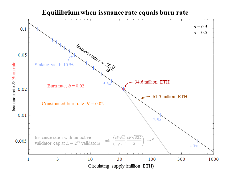
Figure A. The equilibrium illustrated by letting the y-axis represent both the burn rate b (red line) and issuance rate i (black line), with the circulating supply on the x-axis. The grey line indicates the issuance rate with a 2^{19} active validator cap. Circles indicate the equilibrium which is located at the points where the lines for the burn rate and issuance rate cross. The staking yield (excluding tips) is indicated in blue and the constrained burn rate b’ set as 0.02 in orange. Vector graphics for the figure: BurnIssuanceEquilibrium.pdf (147.2 KB)

As evident, the burn rate b and the constrained burn rate b’ differ by a constant factor in the figure. This means that even when the burn rate is reduced by discounting staked ether, there will still be an equilibrium–the burn-rate curve is still independent of the circulating supply and just shifted downwards in the figure. Similarly, yield demand can influence the deposit ratio, shifting the burn-rate curves up and down, or shifting the issuance-rate curve left or right. The relationship between b and b' can be clarified by rearranging the equation for the constrained burn rate

b’ = \frac{B}{S-aD},

b’ = \frac{B}{S-adS},

b’ = \frac{B}{S(1-ad)},

b’ = \frac{B}{S}\frac{1}{1-ad},

and substituting in b

b’ = \frac{b}{1-ad}.

This relationship makes it possible to compute the burn rate for the constrained burn rate as in the example presented in the figure:

b = b'(1-ad) = 0.02(1-0.5\times0.5) = 0.015.

1 Like

I will answer the questions (below) from @CostOfSecurity that were asked on the previous version of this post here instead.

How has this not gotten more attention? This is a great presentation of long-term impact of deflation on ETH supply. I am still working my way through your work again to ensure I fully understand it; but It seems that this is going to have a very significant impact on network activity.

With my initial analysis on this problem, at issuance between 1,800 to 2,600/day the network would only support 600k transactions/day with average base_fee of 18 and 1,000,000 transactions/day with average base fee of 16 respectively. Is this similar to what you estimated?

Perhaps it wouldn’t be as much of a problem with a robust layer 2 settlement activity constituting the majority of L1 transactions.

It also seems that the minimum dollar-denominated market cap will rise linearly with the dollar-denominated economic demand at this equilibrium. Such that the dollar-denominated economic demand would drive the dollar-denominated cost per ETH proportional to the issuance.

Thanks for reading my work! I am not claiming that the network can “support” a certain number of transactions at a particular base fee. Instead, one part of the analysis focuses on how the circulating supply equilibrium can be derived from the total transaction fees and the yield demand for staking. Relating to your question, with the current issuance policy, a certain burn rate will eventually always be balanced by a certain issuance rate. If the network burns a fixed 3.5 % of the supply per year, the issuance rate would eventually reach 3.5 % of the circulating supply. If the burn rate instead is fixed at 1 %, the issuance rate would eventually be 1 %.

The question then is if we want to preserve such a policy if lower validator rewards are sufficient for ensuring security. Phrased a little differently in fiat terms, if the network at a future date burns 10 billion dollars per year and it would be sufficient to issue 4 billion dollars worth of ether for securing the network, do we wish the issuance to be 4 billion dollars, 10 billion dollars, or perhaps somewhere in between? It becomes a matter of balancing the interests of different stakeholders in the Ethereum ecosystem. These questions may not come into play for quite some time since the issuance rate is on track to be much lower than the burn rate initially. It is however good to start the discussion right away.

Your final remark is plausible in the sense that the burn rate can be understood as the income of the Ethereum network but also in some sense as the “earnings”, because it will all be distributed to token holders either through deflation or issuance. Another definition of earnings could be to subtract minimum viable issuance from the yearly burn:

E = B-I_l

I focus here on burn instead of issuance, although they are somewhat coupled, since it is a better way to express intrinsic value: it takes no effort for a blockchain to issue tokens but it is hard to induce demand for paying transaction fees.

I expect to post a pdf with a little more detailed analysis on the supply equilibrium and issuance policy in a while.

1 Like

Thank you for the response. I’ve been thinking more about what you’ve said and have a couple questions/comments.

First, with regards to my comment about transactions per day, I was making a lot of assumptions but was more referring to the burn rates from the current block size and burn mechanism.

From my understanding, the block gas_target is set at 15,000,000; at B = I equilibrium, so on average, the gas consumed per block should be this amount. At a block time of 12 seconds, there should be about 2,628,000 blocks per year; so the total consumed gas per year should be around 3.942x10^13.

Burn (B) = Gas_used * Base_Fee
Issuance (2^19, 2^20) = 681,574 and 963,892 ETH

When I = B; Base_Fee = I/Gas_used

  • at 2**19 validators, average Base_Fee should be 17 (ETH transfer should be 0.00036 ETH)
  • at 2**20 validators, average Base_Fee would be 24 (ETH transfer should be 0.0005 ETH)
  • lately, simple ETH transfer would be around 0.0021 ETH at base_fee rates of 100gwei

This might not be the best analogy, but I think of base_fee as a proxy for volatility in order flow with low base_fee indicating a much more stable gas_consumption market. Thus, as ETH becomes more scarce, I would expect the base fees to stabilize towards these values. I think it is interesting to think about what type of factors would be driving this, as it appears to me, that the ETH cost to transact on mainnet will decrease over time, even if demand increases.

I think this may also be helpful in modeling costs of transactions for the future based on the assumption there will be a limited amount of gas available from issuance. I still have more to think about on this topic but would be interested to hear any of your thoughts.

With regards to minimum viable issuance, it seems that as issuance drops this will lead to further reductions in average base_fee and thus less flexibility in handling fluctuations in transaction volume. While it seems like all of these things will help stabilize the ETH cost of transacting on the network, I think this would translate to a significant increase in fiat-denominate ETH prices as demand changes.

I also wonder if it would be impossible to maintain a desired deposit ratio. I really need to think more about the potential impact of a dynamic reward factor, but I can image that there is a “stable” supply reached at a particular burn rate. However, if the deposit ratio is <1.0, and the demand for the network increases and thus dollar-dominated price, excess supply could be sold and burned in transactions further driving the deposit ratio up.

Than if yield decreases to drive deposit ratio towards minimum viable issuance, the excess supply could then be sold/burned if demand exisits until no ETH exists?

I highly doubt you can obtain a supply equilibrium in this manner. The reason for this is that the network revenues, which in the end determine the burn rate, are an independent variable which is mostly related to how much demand there is for Ethereum blockspace and is best understood as priced in fiat (let’s say USD). This creates an interplay between the network revenues and the price of the ETH token that determines at which regime the network is operating (deflationary, inflationary or no-net token creation).

There are multiple reasons why the network revenues are best understood as priced in fiat:

  • When the fees are too high, low added value transactions get pushed out of the network. Best proof that this is the case is all the people complaining that Ethereum’s fees are too high. When people complain the fees are too high they are implicitly saying that for the USD value of their transactions the network fees are not worth it. This creates a form of auction in that only users that can pay the USD price of the fees for their use case use the network. To be fair there is a bit of reflexivity in the price of ETH and the network revenues in that the native economy doesn’t care as much if the price of the gas fees raises because the price of ETH raises. But this is constrained by next bullet point.

  • Since a large part of the network fees is burnt, over the long-term users of the network will need to keep replacing some of the burnt tokens by acquiring more ETH in the open market. If they don’t they will cease to use the network as they run out of ETH to pay for the fees. So again, this prices the network fees in USD as you need to keep buying the ETH to be used for the network.

What all this means is that the monetary policy of Ethereum is sensitive to the price of the ETH token (and viceversa). For a given use of the network (priced in USD) you can calculate the different monetary regimes of the network separated by a price of the ETH token.

  • Below that price the network operates in a deflationary regime and destroys token, this token destruction process is linear (for a fixed price of ETH and network revenues in USD) which means there is a finite amount of time until all ETH is destroyed which is clearly impossible and will result in a supply crunch forcing the price of the ETH token higher (or perhaps the network revenues to dry down).

  • At exactly that price the network is not inflationary nor deflationary. There is 0 net issuance and the network has achieved supply equilibrium.

  • Above that price the network is inflationary.

We can make a strong argument for the first regime (deflationary) not being sustainable long-term, in the asymptotic future. In fact, you can calculate the amount of time it will take for the entire token supply to be burnt as a function of network revenues and the price of the token. Which is obviously impossible.

By not sustainable I don’t mean to say it’s bad for the network, just that it cannot be maintained indefinitely. Ethereum’s monetary policy and market forces will push the token price higher until the deflationary regime is left behind. For given network revenues there is a price floor for the token and the monetary policy will operate in a way that will guarantee it’s met long-term.

So long term, Ethereum will operate at either 0% inflation or positive (bounded from above by the total issuance). To what extent the inflation rate is positive will depend on Ethereum’s monetary premium. That is, how much extra are market participants willing to pay for an asset with the monetary characteristics of ETH.

But the total circulating supply at which this equilibrium is reached is hard to estimate as it depends on market dynamics (i.e. how the market reacts to the supply crunch of Ethereum’s deflationary regime, plus the ETH demand for its utility and monetary premium).

You can see all of this argued in more detail in the following spreadsheet: Ethereum Price Models - Google Sheets

Good evening and thanks for reading my post! I have a little hard time understanding what you are arguing against. Perhaps you came here from my recent post on r/ethereum and thought that either post specifies Ethereum as being deflationary long term. The post on r/ethereum merely concludes that deflation is economically sound in terms of driving economic activity. It does not argue that Ethereum will be perpetually deflationary. Sections 1-5 of my Ethresearch post details the current policy with an analysis of the equilibrium circulating supply. A circulating supply equilibrium is the same thing as “0 % inflation”, which you in turn argue that Ethereum will operate under. Please note my answers to Barnabé with a more detailed motivation for why the current policy leads to an equilibrium (0 % inflation). However, perpetual deflation is not avoided due to

Rather, it is the way that the issuance depend on the deposit size (and thus the circulating supply) that leads to an equilibrium.

Section 6 stipulates the conditions for how the current policy could be changed to a deflationary policy, if this is desirable. There are good arguments both for and against having a deflationary policy. It is however not true that it cannot be achieved. It can be achieved by maintaining an issuance rate below the burn rate through gradual adjustments of the issuance policy while ensuring a sufficient deposit ratio.

Modeling the circulating supply equilibrium and other aspects of Ethereum’s economy using the burn rate instead of assuming people paying a fixed amount of fiat for transactions has some nice properties. It is also an assumption that needs to be more deeply analyzed and I am currently writing a longer text detailing the fine prints of the assumption. In essence, if the value of a cryptocurrency (total market cap) is reflected in how much people are willing to pay in total each day/week/year for transacting on the network, then this means that the burn rate will be maintained relatively fixed. It can be understood a little like assuming that Mastercard will maintain a rather fixed P/E ratio instead of assuming that they will charge 2.3 dollars per transaction indefinitely. In the short term, a year or two, perhaps this transaction price will be true. But who knows what the situation will look like in 20 years? Perhaps competition or new technologies will push the transaction price to 0.1 dollars or fiat inflation will push it to 23 dollars. And what about in 100 years? To quote Keynes, we simply do not know. But we can make guesses about the P/E ratio also for very long time frames. It is grounded in valuation methods that have stood the test of time.

For Ethereum, it is even harder to make guesses about future fiat denominated transaction prices. Perhaps L2 and L3 scaling will mean that a transaction on L1 can settle thousands or millions of real transactions, making very expensive transactions on L1 economically feasible. Perhaps sharding and state expiry will make it possible to write a lot more data to L1 than what is currently possible. By assuming that the market cap of Ethereum is related to how much people are willing to pay for transacting on it in total, the burden of making correct fee estimates is removed. In essence, by using the burn rate in the models, the token price is implicitly accounted for, relying on time-tested valuation methods. The models can then handle infinite time scales while removing some uncertainties. Of course equity valuation methods must be adjusted to the specific circumstances of cryptocurrencies, but that is beyond the scope of this answer.

Thanks for your reply @aelowsson !

My apologies if I didn’t make my claim clearly stated. What I’m trying to say is that you cannot derive the equilibrium circulating supply from first principles because it’s dependent on exogenous factors outside of control of the network. These factors are; price of the ETH token, and blockspace demand.

These are reflected in your variables through b . This parameter is dependent on the price of the ETH token, demand for blockspace (i.e., network revenues paid as base_fee), total circulating supply. If you know these 3 things you can calculate b, unfortunately two of them are completely outside the control of the network.

In the rest of the post I try to explain that besides making a general statement that in the asymptotic future B < I. We cannot claim (from first-principles) what will be the circulating supply when this is reached. That is, in the very long-term the network must operate in the regime 0 \le inflation < I / S but we cannot say when this will be the case or what will be the circulating supply when inflation = 0 or even if inflation will remain 0, could go higher (I suspect this will be the long-term situation if the network is successful).

Hope I managed to explain better my claim. Perhaps I’m misunderstanding the intent of your post but when I see concrete figures of an equilibrium circulating supply it irks me. And makes me suspect something is not properly understood.

Let me know if I’m misunderstanding something.

You’re welcome :slight_smile:

You are assuming that the price of the ETH token, the network revenue, and the circulating supply have no relation to each other but that is not resonable. It is like saying that you cannot guess how old a randomly selected human in the history of humanity became because you do not know the date of birth and the date of death. These two variables will be related to each other through the human life expectancy, thus giving a plausible range of 0-120 years. Let us circle back to the example with Mastercard. Do you agree that the following circumstances apply 50 years from now?

  1. We cannot know the number of oustanding shares.
  2. We cannot know the price of one Mastercard share.
  3. We cannot know how much the company will earn each year.
  4. We can still make a ball-park estimate of Mastercard’s p/e-ratio (a crude proxy for the burn rate in this example) 50 years from now. It will likely hover somewhere between 7 and 70. There will be some good years and some bad years or decades where this is not true, but that is the p/e ratio that Mastercard is likely to return to should it continue to function as a viable company. If the p/e-ratio goes below 7, investors will buy shares to get a slice of the earnings, pushing the p/e-ratio back up. If the p/e-ratio goes above 70 with no viable path to improve profitability, investors will sell shares pushing the p/e-ratio back down.

Using the same reasoning, if the burn rate rises above some specific number, say for example 0.06, the strong buy pressure from those seeking to capture the staking yield will push up the ETH token price until the burn rate is reduced (too expensive to transact). If the burn rate becomes very low, there will eventually be a sell pressure on the ETH token, pushing the burn rate upwards (cheap to transact). That is assuming that Ethereum is still a viable network.

The assumption of the equilibrium is thus that the fiat denominated yearly burn will not detach from the fiat denominated market cap.

EDIT:
I removed my imprecise remarks regarding b and raising F and have made a new reply (the next in this thread) that illustrates the situation if the burn rate becomes very low, i.e., that the revenue detaches from the market cap of the chain. I came to realize that in this case it is actually possible to define the lowest burn rate that leads to a circulating supply equilibrium, based on assumptions about the other relevant variables.

If you studied my post you will see that I derive the equations for computing the equilibrium so that we can get a better understanding of the economic forces operating within Ethereum. This gives us the tools necessary to design the network in a way that is sustainable long term. The end goal is not a precise estimate of the circulating supply (nor the token price). The figures in Sections 3-4 are exploratory precisely because of the great uncertainty. We cannot know what yield stakers will be satisfied with and we cannot know what the exact burn rate will be going forward. People can use the plots to see how the circulating supply equilibrium varies with yield and burn rate.

The same for the figure in my response to Barnabé that illustrates the equilibrium with burn rates between 0.003-0.1. I am currently devising a probability distribution estimate for the circulating supply which I think will better highlight the great uncertainty.

Did you understand the effect of the issuance policy and how it acts to push the network into an equilibrium, as further detailed in my answers [1, 2]?

2 Likes

Actually the circumstances where participants decide to raise F does represent a break from the equilibrium, pushing the circulating supply upwards. But this situation emerges only when the burn rate is many times lower than yield. The requirement is that the yield is too low to motivate staking above the lowest deposit ratio that is acceptable for security (d_l).

The equation from Section 5.3 for the relationship between d, b and y at the equilibrium can be used to analyze this situation. For example, it is possible to compute the burn rate that will lead to d < d_l given d_l and y_l (the stabilized yield at d_l). For example, if d_l = 0.07 and y_l = 0.01, then the minimum burn rate b_l that supports a circulating supply equilibrium (no raise of F) is

b_l=d_ly_l=0.07\times0.01=0.0007

In other words, with the given assumptions about d_l and y_l, a burn rate around 30-40 times lower than the current burn rate could lead to a need for increasing F. That would bring up the yield but also means that the circulating supply will start rising, over time putting a downward pressure on the yield. Thus, should circumstances that lead to d < d_l remain, (i.e., b < 0.0007, stakers demand more than 1 % at d_l to stake) the network will end up in the same situation again down the road, and will have to continue raising F to produce inflation that satisfies an acceptable deposit ratio. This thus sets a bound on b for retaining a circulating supply equilibrium.

I made a figure that attempts to visualize this relationship between S, i, b, d and y at the circulating supply equilibrium. It uses the same values as in my example above, illustrating the situation in the bottom right corner if the burn rate is below the blue line indicating 1 % yield at a deposit ratio of 0.07 (indicated in green). The average b since the start of EIP-1559 (as of the end of March) is indicated in the upper left corner. The deposit ratio shifts the issuance rate up and down at a specific circulating supply. The blue lines indicate how the yield varies with deposit ratio and circulating supply.

2 Likes

A recent Reddit discussion has led me to this excellent post by Anders. Having discussed with him and @JustinDrake on twitter, I thought I would write down my thoughts on my blog, as well as post the main points here for wider discussion. (link to my blog post)

TLDR, similar to @barnabe 's question (more than 2 years ago :), while I agree with @aelowsson that the issuance and burn has opposing effects, it is hard to conclude there will be an equilibrium (or inflationary, or deflationary) on ETH’s total supply. Reason being the issuance and burn operates in two different markets (not sure if @aelowsson’s updated paper will address this point, very much look forward to the new paper).

To clarify further:

  • Burn is driven by blockspace supply-demand.
  • Issuance is driven by staking demand, which is primarily dependent on staker’s perceived view of ETH as a long term SoV.
  • Burn is a utility market. Issuance is a SoV market.
  • A thought exercise to illustrate this: when long term SoV investors stake their ETH, how much do they care what the current burn rate is? It is unlikely to be the main consideration. Hence the comparison to mastercard PE ratio above is flawed, since mastercard share is an investment product, not an utility, you don’t buy mastercard shares to use the mastercard network. There is a single market of supply-demand for mastercard share, unlike the ETH supply-demand dynamics with two separate markets.

Let’s consider a more concrete example:

  1. Assume an initial state of equilibrium, issuance rate = burn rate
  2. Some external forces break the equilibrium, such as faster adoption of ETH as SoV leading to more investors holding and staking their ETH. ETH’s fiat price increases due to increased demand. More staking also leads to issuance rate increase.
  3. Does the increased ETH price lead to an increased burn rate that offsets the increased issuance rate?
    a). Burn rate may stay the same. e.g. although transaction spending in fiat terms has increased, most transactions may be L2 settlements with higher economic value.
    b). Or burn rate may decrease, e.g. transactions are too expensive in fiat terms.
    c). Or burn rate may increase,e.g. the hype of ETH as SoV help to stimulate the network usage

We may conclude 3c) is most likely. The question then becomes how to model if and when the two changes will converge? (if there is a mathematical relationship that implies the burn rate and issuance rate will always converge, I am eager to know)

A more likely scenario is that ETH will be alternating between periods of (low)deflation and (low)inflation, depending on factors such as blockspace supply growth (L2) and demand, market cycle (both crypto and traditional market), competition for SoV assets etc. Further work is needed if we want to further model it out.

Finally, the above analysis is based on the current protocol issuance design, future research such as validator cap, update to the issuance formula etc will change the dynamic.

My post above is from a theoretical point of view.
In practise, let’s look at where the network will develop from here.


Given the on-going research on the max number of validators , resulting in ETH deposit limit of 2^25 - 33.5m. At the current avg staking deposit rate of 20k ETH per day, it will take almost 3 years to reach the 33.5m deposit limit. We can safely assume that the staking amount will reach this limit, given the SoV appear of ETH the asset, plus the prevalence of LSD meaning even staked ETH can still indirectly participate in the crypto-economy.

As shown in the table above, even at moderate gas base fee of 25 gwei, the network is still deflationary. So if you believe the network average gas fee will be above 25 gwei (remember this is half the average since 1559) , then Ethereum will be deflationary within the next 3 to 5 years. Afterwards a new period will begin where Ethereum will be alternating between periods of (low)deflation or (low)inflation, depending on factors such as blockspace supply growth (L2) and demand, market cycle (both crypto and traditional market), competition for SoV assets etc.