Data availability proof-friendly state tree transitions

[musalbas]

Problem

State trees are an important element in a blockchain that supports fraud proofs or stateless clients, because they are needed to prove that a) a fraudulent transaction is attempting to spend an input that does not exist (in a UTXO-based blockchain), b) a fraudulent transaction is performing a transaction based on state that does not exist (in an account-based blockchain) or c) in the case of a stateless client, prove that some state exists.

However, a malicious miner could create a blockchain with a fraudulent state tree root, that does not match the state transitions made by the transactions in the block, and so no one would be able to find prove the inclusion of any state in the tree and find proofs of fraudulent state, because they don’t have the data for it. You could prevent this by having data availability proofs for the entire state tree, but it would of course not be efficient to require nodes to broadcast the entire state of the system every block.

Solution abstract

A solution to this is to have many “intermediate” state tree roots, and corresponding merkle proofs for all the intermediate state tree roots that show modifying the state tree in a certain way should lead to the next intermediate state tree root. If any of these intermediate roots are wrong, then fraud proof is limited to that specific intermediate root.

Solution design

Each block header contains a standard sparse merkle tree with 2^{256} leafs (every possible SHA256 hash), such that a leaf at index k represents the state of the key k (if you don’t understand how having 2^{256} leafs is even possible without burning the universe, see the linked paper). Sparse merkle trees are used because they do not have to be rebalanced, so if you have tree A and tree B, where tree B is tree A but with one leaf that is different, then proving that the root of tree A becomes the root of tree B when you change a specific leaf is always O(log(n)). I will call this a “merkle change proof”: which is a merkle proof that the root of tree A, combined with some change in leaf index k in tree A, makes the root of tree B.

Now, instead of publishing just one sparse merkle tree root in each block header, a miner should publish multiple intermediate tree roots in the same header, such that, for example, if you apply the results of transactions 1-10 to the previous block’s sparse merkle tree root, you get intermediate root R_1, then if you apply transactions 11-20 to R_1, you get intermediate root R_2, until you apply all the transactions to each previous root and get final root R_n.

Because there is an implicit ordering to the transactions in a block, a full node can now easily generate efficient fraud proofs for invalid state roots, because they only have to prove that one intermediate root is invalid for the whole block to be invalid. If a full node applies transactions 1-10 to the previous block’s sparse merkle tree root, but does not get the same intermediate root R_1, then they can publish a fraud proof, which will consist of a merkle change proof that applying transactions 1-10 to the previous block’s sparse merkle tree root does not result in the published root R_1. The same can be repeated for R_1 and R_2, R_2 and R_3, and so on.

The maximum size of the fraud proof is therefore equivalent to the number of transactions added by each intermediate state root (in this case, 10). However, light clients also need to be sure that the intermediate roots are actually available for full nodes to generate fraud proofs for, so these intermediate roots should be included in the same block of data that is covered by any data availability scheme such as erasure coding. This means there is a tradeoff between the size of the fraud proof, and the size of the data (the intermediate roots) that light clients need to ensure availability for.

[vbuterin]

It’s worth clarifying that you don’t need a sparse merkle tree to just do intermediate state roots and proofs of execution / fault proofs, though; a Patricia tree fully suffices for that. You are right that binary sparse merkle trees are much more friendly to data availability proofs, but there are two issues with this:

• Proofs in sparse merkle trees are significantly longer, ~32 * 160 = 5120 bytes instead of ~32 * log(N) ~= 960 bytes at 1B accounts for a binary Patricia tree.
• Actually doing erasure coding on a large state will take a very long time, and recalculating erasure code data will also take a very long time even if the state only changes slightly.

[musalbas]

@vbuterin

Proofs in sparse merkle trees are significantly longer, ~32 * 160 = 5120 bytes instead of ~32 * log(N) ~= 960 bytes at 1B accounts for a binary Patricia tree.

You don’t need 160 hashes for a sparse merkle tree inclusion proof, because almost all of the leafs will have default values, so these hashes don’t need to be specified explicitly. E.g. most level 2 nodes will have the value H(0 || 0), most level 3 nodes will have the value H(H(0 || 0) || H(0 || 0)), etc. So it’s still about ~32 * log(N).

Also of interest: Efficient Sparse Merkle Trees (and implementation)

[vbuterin]

Ah, but if there’s an object C at some particular address, say, …01011, then the nodes above it are:

• H(0 | C)
• H(0, H(0 | C))
• H(H(0, H(0 | C)), 0)
• H(0, H(H(0, H(0 | C)), 0))
• H(H(0, H(H(0, H(0 | C)), 0)), 0)

The values along the branch are unlikely (read: never) going to be repeated.

[vbuterin]

Aaaaah, I suppose that you could compress the branch by saving it in the form (…01011, C), and then letting clients recompute it as needed.

Actually, now that I think about it, this could the start of a much better kind of state tree…

[vbuterin]

OK, you’re absolutely right. It is definitely possible to store the entire state in a sparse binary Merkle tree, with 2**160 nodes. There are two key tricks needed for this to happen:

1. Setting up an initial (empty) trie. Every bottom level node is 0x00 * 32. If every level N node is X, every level N+1 node is sha3(X + X). Hence, you can calculate the root hash and intermediate nodes of an empty trie with only 160 rounds of computation.
2. Compressing a Merkle branch for a value. One disadvantage of this kind of tree is that the length of a Merkle branch considered naively is much longer than it is for a Patricia tree; a binary Patricia tree with N nodes has an average Merkle branch length of ~32 * log2(N) bytes in theory, and about 10% more in practice because of overhead, but a sparse binary tree would have a Merkle branch length of ~32 * 160 bytes, or even more if we decide to increase the address length. But this can be solved if we notice that for most of the Merkle path, the subtree being considered will have only one node, and so the opposite node (ie. the node that would go into the proof) is a node of an empty subtree. There is only one possible hash for an empty subtree at any given height, so this can be compressed down to one bit.

A Merkle proof length could be fairly easily shortened to 64 + 32 * log2(N) bytes, where the 64 bytes of overhead consists of (i) the key, and (ii) 256 bits where the ith bit represents whether the ith opposite node should be read from the Merkle proof or taken as the empty subtree root for that height; this is comparable data overhead to the existing binary Patricia tree and can be further optimized if needed.

The key benefit here is a massive gain in simplicity. Here’s a code implementation of get/set and Merkle proof creation and verification:

def new_tree(db):
    h = b'\x00' * 32
    for i in range(256):
        newh = sha3(h + h)
        db.put(newh, h + h)
        h = newh
    return h

def key_to_path(k):
    o = 0
    for c in k:
        o = (o << 8) + c
    return o

def get(db, root, key):
    v = root
    path = key_to_path(key)
    for i in range(256):
        if (path >> 255) & 1:
            v = db.get(v)[32:]
        else:
            v = db.get(v)[:32]
        path <<= 1
    return v

def update(db, root, key, value):
    v = root
    path = path2 = key_to_path(key)
    sidenodes = []
    for i in range(256):
        if (path >> 255) & 1:
            sidenodes.append(db.get(v)[:32])
            v = db.get(v)[32:]
        else:
            sidenodes.append(db.get(v)[32:])
            v = db.get(v)[:32]
        path <<= 1
    v = value
    for i in range(256):
        if (path2 & 1):
            newv = sha3(sidenodes[-1] + v)
            db.put(newv, sidenodes[-1] + v)
        else:
            newv = sha3(v + sidenodes[-1])
            db.put(newv, v + sidenodes[-1])
        path2 >>= 1
        v = newv
        sidenodes.pop()
    return v

def make_merkle_proof(db, root, key):
    v = root
    path = key_to_path(key)
    sidenodes = []
    for i in range(256):
        if (path >> 255) & 1:
            sidenodes.append(db.get(v)[:32])
            v = db.get(v)[32:]
        else:
            sidenodes.append(db.get(v)[32:])
            v = db.get(v)[:32]
        path <<= 1
    return sidenodes

def verify_proof(proof, root, key, value):
    path = key_to_path(key)
    v = value
    for i in range(256):
        if (path & 1):
            newv = sha3(proof[-1-i] + v)
        else:
            newv = sha3(v + proof[-1-i])
        path >>= 1
        v = newv
    return root == v

[musalbas]

Cool! There’s also the advantage of a better balanced tree, no?

Regarding the idea of doing fault proofs using intermediate state roots, I came across a cute little result. When you have a scheme where you need to assign some data into chunks (in this case, we’re chunking transactions into intermediate state roots), you can always achieve O(\sqrt{n}) computational complexity by arranging the data into a square. (This applies to the two-dimensional erasure coding scheme, too.)

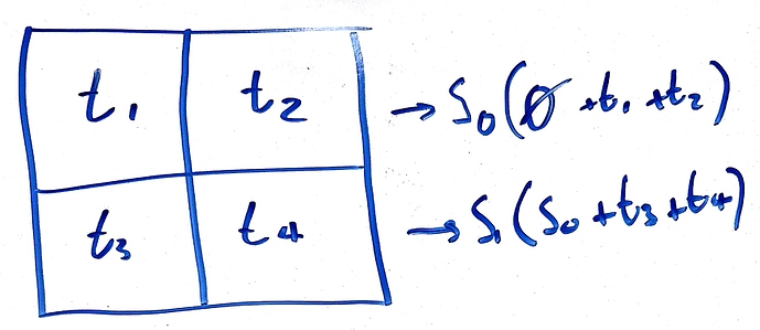
Suppose we arrange the transactions into a square, and we generate an intermediate state root for each row, such that the intermediate state root for each row is the state root that is generated upon applying all the transactions in that row to the intermediate state root of the previous row.

Here’s an illustration (s_i represents the intermediate state root for row i, and t_j represents a transaction, and s_i + t_j represents the new state root that you would get if you apply t_j to s_i):

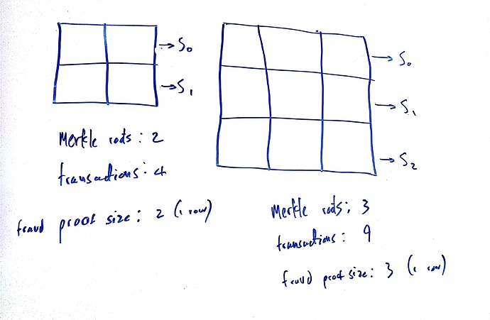
By arranging transactions into a square, each intermediate state root deals with \sqrt{n} transactions for n total transactions. Additionally, the number of intermediate state roots in the square is also \sqrt{n}. This means that the number of merkle roots required for download by light clients, as well as fraud proofs for intermediate states, are both \sqrt{n}. Here’s an illustration:

[vbuterin]

But isn’t that just making a Merkle tree on top of a Merkle tree, which is basically the same thing as having a bigger Merkle tree?

If the goal is to be able to do erasure coding checks on rows and columns, then as I say in the post it can work, but it requires Merkle roots for both rows and columns, and a fraud proof mechanism for capturing inconsistencies between the two.

[MaxC]

I think, instead of using a 2-d erasure code, you can just split a file into root(n) chunks and erasure code each chunk. There is no real need to have a 2-d erasure coding for columns and rows, and capture consistency between them.

[musalbas]

@vbuterin

But isn’t that just making a Merkle tree on top of a Merkle tree, which is basically the same thing as having a bigger Merkle tree?

If the goal is to be able to do erasure coding checks on rows and columns, then as I say in the post it can work, but it requires Merkle roots for both rows and columns, and a fraud proof mechanism for capturing inconsistencies between the two.

Yes but the point is that the number of Merkle roots a light client needs for rows and columns is 2\sqrt{n} for n transactions, because the length of a row (the side of a square) is \sqrt{n}. Hence O(\sqrt{n}) complexity.

I don’t follow what you mean about a Merkle tree on top of a Merkle tree. Each intermediate state tree is a single tree, that is constructed based on the previous intermediate state tree and the next transactions in the block, in order. Hence creating “snapshots” of the tree that can be used as a proof of execution of the state tree transitions being applied correctly, allowing full nodes to generate fault proofs.

@MaxC

I think, instead of using a 2-d erasure code, you can just split a file into root(n) chunks and erasure code each chunk. There is no real need to have a 2-d erasure coding for columns and rows, and capture consistency between them.

I don’t think that results in the same properties, because instead of randomly sampling chunks from the whole square, you’d need to sample some chunks from every root(n) piece, to have some assurance that the data behind every root(n) piece is available.

[MaxC]

@musalbas

I think, instead of using a 2-d erasure code, you can just split a file into root(n) chunks and erasure code each chunk. There is no real need to have a 2-d erasure coding for columns and rows, and capture consistency between them.

Even if you randomly sample chunks from the whole square, to generate a succinct fraud proof from a 2d erasure code, you need root(n) values from a row or column. So if you want to guarantee succinct fraud proofs, you still need to check the availability of each row and column.

[musalbas]

Generating a fraud proof and probabilistically checking the availability of the square are two different things though.

If you don’t have rows and columns, and only root(n) pieces, all you’re really doing is splitting up the block into multiple microblocks with different erasure codes. If you want to hide any data from the entire block, instead of needing to hide 50% of the block, you only need to hide a few % of the block (i.e. half a microblock), so you need to randomly sample a lot more chunks.

[MaxC]

Hmm, I’m not so sure.

Generating the fraud proof is one side of the coin. Checking availability is the other. the point being you can’t reduce the fraud proof size without increasing the amount of checking.

Two cases:
(Worst case analysis, assuming an adversary will try to force the largest fraud proofs)
(1) You check all O(root(n)) merkle roots for 2-D erasure code, and only then will the code offers the same guarantees as having a merkle root for each microblock. => root(n) size fraud proofs.
(2) You don’t check all roots, and then a 2-D code has the same guarantees on fraud proof size that checking just a single merkle root for the whole block does. => O(n) sized fraud proofs, and you may as well just use a 1-D code for the block.

[musalbas]

You don’t have to randomly sample from all O(root(n)) rows and columns in a 2D erasure code though, you randomly sample from the entire square, and you can miss rows and columns while randomly sampling. According to my rough calculations, if you want to hide a single chunk in the square, you’d have to hide about 25% of the square (draw it out to see what I mean). With microblocks, you only have to hide half a microblock (a few % of the entire block).

[MaxC]

@musalbas

You don’t have to randomly sample from all O(root(n)) rows and columns in a 2D erasure code though, you randomly sample from the entire square, and you can miss rows and columns while randomly sampling. According to my rough calculations, if you want to hide a single chunk in the square, you’d have to hide about 25% of the square (draw it out to see what I mean). With microblocks, you only have to hide half a microblock (a few % of the entire block).

For clarity, could you let me know what value you are calculating for the i,j th entry of your 2-d erasure code? what you suggest seems to be contrary to the docs:

In such a model, we add some further complexity to the data structures involved. First of all, instead of having a single Merkle root, we now have 4 * sqrt(M) Merkle roots, one for each row and one for each column. Light clients would need to download all of this data as part of a light client proof…

A major benefit of this is that the size of a fraud proof is much lower: a fraud proof now consists of M values in a single row or column plus Merkle proofs for these values

[musalbas]

See the “Going Multidimensional: The Self-Healing Cube” section in https://blog.ethereum.org/2014/08/16/secret-sharing-erasure-coding-guide-aspiring-dropbox-decentralizer/.

The fraud proofs consist of a single row or column, but that doesn’t mean you have to sample from every single one. Even if an entire single row is missing, you can recompute it from the columns.

[MaxC]

Thanks for sharing. That is very interesting but you’d still need root(n) columns to reconstruct the row, so wouldn’t the fraud proof still have O(n) size?

Might be possible with crypto-economics- i.e. I claim that the values in m=root(n) columns are x_1...x_m, which forces a row to be some value, s. Then the erasure code creator can challenge any one of these claims, say x_1 wlg. In the event of a challenge, I have to then produce the signed merkle root for values y_1 ...y_m producing x_1?

This process can go on and on until termination. The question is how many rounds would be needed on average.

[musalbas]

Good question, if an entire row is missing, I’m not sure how you’d construct a fraud proof to show that a specific row is inconsistent with its merkle root, without having to show all of the columns in the fraud proof so the light client can reconstruct that row for themselves.

[MaxC]

Should be possible crypto-economically, but would like to look into it more in depth.

[musalbas]

Oh actually, it’s quite simple. If an entire row is missing, the fraud proof consists of M merkle proofs of the missing chunks of the rows recomputed from the columns, from the column merkle roots. The light client then computes the whole row from these column merkle proofs, and checks to see if it matches the given merkle root of the row. There’s quite an overhead for having to provide a merkle proof for every chunk, though.

You could also make it so that when a client randomly samples an (x, y) chunk in a square, they must receive a merkle proof from both the column and row roots, which makes inconsistencies between rows and columns more difficult to get away with.