Deep dive into Current PoW Difficulty Adjustment Algorithm and a Possible Alternative

TL;DR
In the difficulty adjustment algorithm for Homestead the scalar represented as max(1 - (block_timestamp - parent_timestamp) // 10, -99) scales linearly based on the blocktime when the probability that a certain blocktime occurs is based off of an exponential function. This is a mismatch and has interested me for some time. Recently, returning to the problem and after learning they are represented best by a Poisson Point Process I have a theory you can use this fact to build a different, simpler, algorithm that also better fits the probability distribution. Hopefully this means better responsiveness and less unnecessary adjustments. I am unsure, but I am at the point where I could use help simulating different cases. Anyone interested in helping me out on this? A deeper explanation of the discovery and possible solutions below.

Intro

Previously at the Status Hackathon before Devcon last year, Jay Rush and I researched the effects of the time bomb on the up and coming fork. During this time I also noticed that the distribution of observed Blocktimes wasn’t normal. It followed some kind of exponential distribution but not exactly. Lucky for me Vitalik pointed out that this is because it is a Poisson Point Process + a Normal Distribution based on block propagation in the network. I view it as each miner is a racehorse, but the horse only runs after he hears the starting pistol. For each miner the starting pistol is the previous block and it takes time for that “sound” to get around.

Mining is Poisson Point Process because each blocktime is completely independent from the previous block time. This leads to a Poisson Distribution which wikipedia has a better explanation than I can write.

In probability theory and statistics, the Poisson distribution named after French mathematician Siméon Denis Poisson, is a discrete probability distribution that expresses the probability of a given number of events occurring in a fixed interval of time or space if these events occur with a known constant rate and independently of the time since the last event

Data

This is the Distribution of just under 10000 blocks spanning from Sept 7th to Sept 8th 2018. Thank you Jay Rush for this! I still have the data from when we worked on the Time-bomb together. It plus the charts below are available on the Google Sheet I used to prepare for this post.

Block%20Time%20Distribution|200px

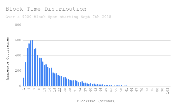
You can see after 3 seconds there is some kind of exponential curve. This in isolation isn’t very interesting, but if you look at this and at how the difficulty adjustment algorithm adjusts to block times it gets a lot more interesting.

Difficulty%20Scalar%20Based%20on%20BlockTime%20(1)

The Formula

    block_diff = parent_diff + parent_diff // 2048 * 
    max(1 - (block_timestamp - parent_timestamp) // 10, -99) + 
    int(2**((block.number // 100000) - 2))

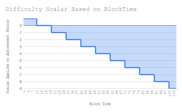
Here you can see that if the blocktime (hereafter bt ) is less than ten it adds parent_diff // 2048 * 1. The 1 in this changes for every bucket of 10. If the previous blocktime is >= 40 and < 50 then the scalar is -3. Or, is subtracts parent_diff // 2048 * -3. At a bt > 1000 this scalar is capped at -99. A great stackexchange post that goes into this further

This is clearly a linear relationship.

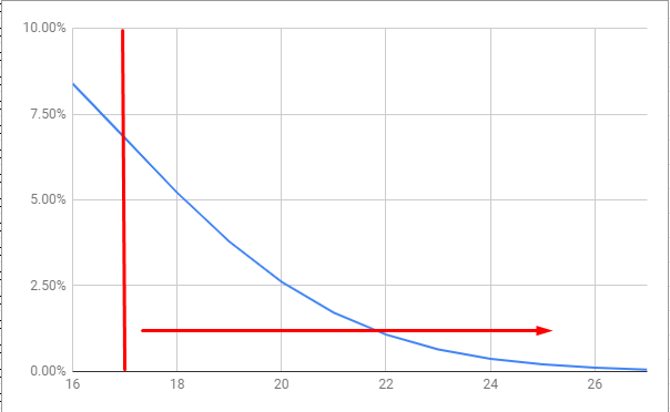
Now lets look at the distribution of blocks within each of these buckets. Here I also add an exponential line of best fit. I understand that this isn’t enough data to get the real values of these probabilities, but it is fairly good estimation. And, the important relationship is shown where the linear adjustment doesn’t match the exponential distribution.

Distribution%20Percentages

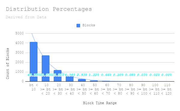
It is easier to see this side by side.
Distribution%20PercentagesDifficulty%20Scalar%20Based%20on%20BlockTime%20(2)

So is there another approach?

First I want to say that this isn’t a proposal expecting to change Ethereum’s Difficulty Adjustment Formula. I want to understand it fully and then publish my findings. That is all. And, perhaps write an EIP for the experience of writing one. I don’t know the real world affects of this mismatch and if it is a real problem or not for the current chain. I also understand most of the focus here is on Serenity which doesn’t have any of these problems. That being said, this is where I have gotten so far.

Start from the Poisson Point Processes you want to see.


A homogeneous Poisson Point Process is completely characterized by a single number λ [1 page 23]

λ is the mean density. In the case of block times it would be the average number of blocks per some unit of time. What is nice about this distribution is you can calculate the probability of occurrences in a given time period.

image

e = Euler's number 
λ = average number of events per interval 
k = number of events occurred

In our collected data above block time was an average 14.5 seconds per block. Some example calculations from this number.

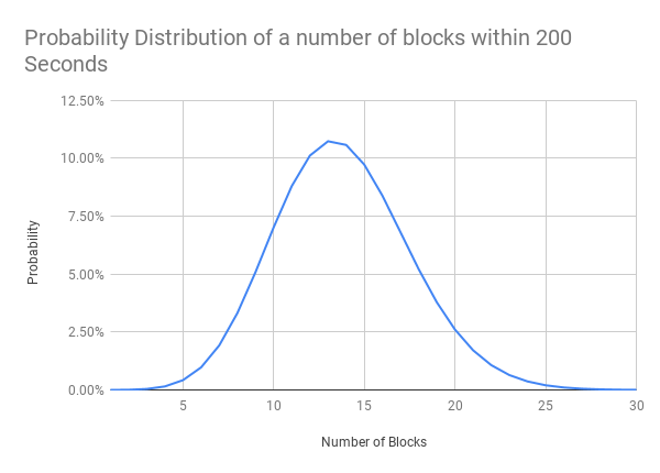
Within 200 seconds what is the probability we would see n blocks.
(λ = 200/14.5 = 13.8)
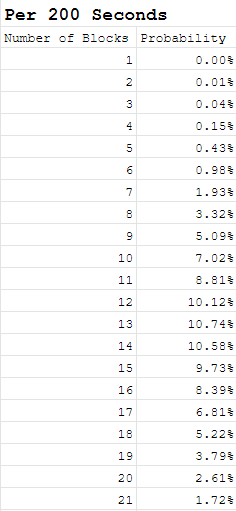
Probability%20Distribution%20of%20a%20number%20of%20blocks%20within%20200%20Seconds

We can also ask:

  • What is the probability there will be between 10 and 16 blocks within a 200 second period?
    • 65.4%

Now given this information we can also ask this in reverse. Given a set of data from a Poisson point process what is the probability that the mean is λ? Or in Ethereum Terms given the number of blocks within a fixed time period what is the probability the average blocktime is 14.5?

I will note this is due to it being a Marked Poisson Point Process and the Marking Theorem described briefly below.

image
An illustration of a marked point process, where the unmarked point process is defined on the positive real line, which often represents time. The random marks take on values in the state space S known as the mark space . Any such marked point process can be interpreted as an unmarked point process on the space {\displaystyle [0,\infty ]\times S}. The marking theorem says that if the original unmarked point process is a Poisson point process and the marks are stochastically independent, then the marked point process is also a Poisson point process on {\displaystyle [0,\infty ]\times S}. If the Poisson point process is homogeneous, then the gaps in the diagram are drawn from an exponential distribution. [2] - Marked Poisson point process

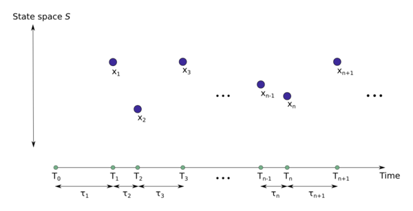
The graph above is similar to plotting blocks over time. The following is a chart of the blocks over constant time (seconds) starting with the block found on Sep-08-2018 01:26:20 PM

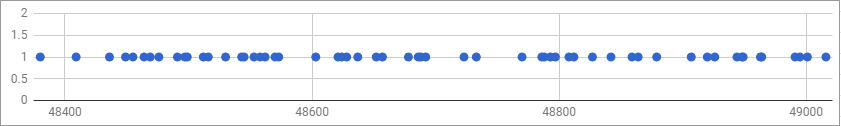
Given any block we can look backwards at the last 200 seconds and observe the probability that currently λ is 14.5. If it isn’t then that means the difficulty is not tuned properly. In the graph above three sections are conveniently segmented. Below I counted the number of blocks and noted the probability
of this many blocks being found based on λ = 14.5

  • 48400 - 48600 : 20 Blocks - 2.61%
  • 48600 - 48800 : 18 Blocks - 5.22%
  • 48800 - 48900 : 17 Blocks - 6.81%

Not particularly useful, as a 6.81% likelihood is not enough confidence to assert λ is in fact not 14.5. In practical terms asserting that the current block difficulty should be changed. But, If in case you use a range like the before mentioned between 10 and 16 blocks there is a 65.4% probability. Stated inversely, if there is less than 10 or greater than 16 blocks, there is a 65.4% likely hood λ isn’t 14.5. This means when adjusting the difficulty outside of these ranges you are, more often then not, correct to do so. A sufficient answer to the question “Should the algorithm change the current difficulty?”.

My theory is there is an ideal length of time to check such that

new_difficulty = parent_difficulty + parent_difficulty*scalar

Where the scalar is defined by the probability an observed number of blocks within a previous x seconds has a λ equal to a Target Blocktime.

This is where I believe simulation and testing would give good enough observable results to decide on ideal values for a target λ. This and as well as more rigorous maths narrowing testing ranges for:

  • Different period lengths
  • Different adjustment thresholds
  • Magnitudes of adjustment

A more specific example.
In the case greater than 17 is selected as the upper adjustment threshold. The scalar can be defined to increase in magnitude proportional to the following equation.
image
The difference of the scalar between 18 and 20 would be nearly a 2x increase. This would much more closely resemble the exponential distribution in observed blocktimes.

Using this method I hope to document a practical alternative to targeting a blocktime for a PoW chain. One that is simple to calculate as well as follows more closely the actual distribution found in blocktimes.

Please any feedback from mathematicians, statisticians, computer scientists, or interested parties would be appreciated. As well as anyone willing to look at testing and simulation implementations. I also have no idea if this bares anything on the beacon chain found in Serenity. Which if it does, I would love to know.

Cheers,
James

References and Sheets


  • [1] Page 23 - Homogeneous Poisson Point Processes
1 Like

Great work!

I will warn that no change is likely to be made in practice, simply because the current adjustment formula is “good enough”, there’s a goal of minimizing protocol changes that don’t have high impact for improving scalability/sustainability, and we are planning a switch to proof of stake anyway.

But it does look like it’s a significant improvement in theory if very rapid adjustment is a goal.

2 Likes

Thank You!

I anticipated as much. It has been on my mind for some time and I didn’t know quite where better to share. Improvements in areas with greatest impact is more than understandable. Especially for Eth 1.x. Thanks for taking the time to check it out. :slight_smile: It is nice to hear feedback it is at least in a good direction.

I am not sure I want to go through the process of writing an EIP for it given how very unlikely it is to be implemented, but it feels good to have thought it through and written it out this far.

Worked with Hawkes Processes and Poisson Point Processes in the past, have been thinking along a Beta distribution however to capture second order statistics so as to have an estimator on conditional variance. From what I’ve read the difficulty adjustment is modeled after simple hysteresis and does its job well.

I’ve found it useful to see the demand and supply side of a given resource as distributions of utility rather than a single point estimator. Not only does this make more sense, but it allows for iterative market-clearing price formation.

A reference on some of the information economics:
Grossman and Stiglitz - On the Impossibility of Informationally Efficient Markets (slides)

I have taken a very market-driven view of turnover within the space.

@vbuterin I really enjoyed your presentation at Eth1.X on the new fee structure. I was the one that had the question about targeting Uncle Rates. If it comes to a point where that is revisited this mechanism may be a good way to do just that. Summarized as follows:

  • Change TARGET_BLOCK_TIME based on Uncle Rates for some period of past blocks.
  • With a MAX_BLOCK_TIME for safety.
  • Increment or Decrement the TARGET_BLOCK_TIME slowly.

Your fee adjustment mechanism paired with a Blocktime re-targeting mechanism may be a good way to maximize “instructions per minute” for the network. Also, it would reward network optimizations immediately that can be done off-chain because the BlockTime can adjust to along the way. The chain operating as fast as is healthy

This is all assuming state size has been defeated of course.

Why isn’t a simple moving average used for difficulty?

Interesting! In physics, it is quite common to approximate functions using Taylor series. I expect that a mathematically exact solution to the difficulty adjustment problem can be reduced to a linear approximation. That would show that the current system is a good approximation assuming the variation in mean block time is low.

Some basic calculations here:

Let’s say we want to target a certain λ’. If we take a long enough time period T, the amount of blocks in that time period N(T) will be equal to the expected amount of blocks for the current E[N(T)]. E[N(T)] = λT = N(T). That means we can compute the current λ = N/T. We want to target a certain λ’, but we can only change it indirectly, via the difficulty. The relation is not direct, there might be unexpected game theoretical consequences when the difficulty changes. For example, some miners might not be profitable and turn off after a certain difficulty. However, for small changes the effect will be linear; the expected number of events in a time period changes inversely with the difficulty. Therefore, the difficulty should be multiplied by a = λ/λ’ = N(T)/λ’T = N(T)/E’[N(T)]. Here E’[N(T)] is the expected number of blocks in time period T given a λ’.

For larger fixed values of T, the difficulty will change slowly and the number of blocks will be close to the expected value.

To see how this relates to the current system, we can also keep N = 1 and make T a variable t to obtain a(t) = 1/λ’t. We can expand it into a Taylor series around λ’ = 1/t, for when the difficulty is nearly correct. The Taylor series becomes a(t) = 1 - λ’(t - 1/λ’) + … Taking the first order approximation and using the target block time t’ = 1/λ’, it can be reduced to a(t) = 1 - (t - t’)/t’. In other words, we obtain the negative linear relationship. Written slightly more familiarly: D’(t) = D + D(t’ - t)/t’.

@ThomasdenH I’ve worked difficulty a lot. Your derivation is problematic because if 1/λ’t = T/t had been used instead of the Taylor series approximation, the results would not have been as good, so something is wrong with the theory. This is maybe because your E’[N(T)] may need to make use of the Erlang distribution (a specific type of Gamma distribution) to get the correct “expectation” for small N like 1. I mean “expected” not in the sense of mean, but what we expect a single block solve time to, given Poisson is more likely to be less than mean as opposed to greater than. Your result with the Taylor series approximation (that accidentally made it a lot better) is the same (for the case of N=1) as Ethereum and another algorithm that also uses the Taylor series approximation and it gets more accurate if you don’t use the Taylor series. The general form of it is the same as Ethereum’s (which I did not realize before):

diff = parent_diff*(1+1/N - t/T/N)

where I use the notation T = 1/λ’ = target solvetime and t= solvetime for previous block. N is a “buffering” factor like the averaging window on a difficulty algorithm, smoothing out the result but making it slower to respond. It’s not valid for small N because it can give negative difficulties. A slightly different derivation to prevent this inverts it and swaps the negative sign:

diff = parent_diff / (1-1/N+t/T/N)

The above comes from using Taylor’s approximation e^x = 1+x+ … in the following difficulty algorithms: :

b = T/t, t=solvetime, T=target time, N=extinction coefficient aka “mean lifetime”.
diff = parent_diff * ( b+(1-b)*e^(-1/b/N) )
and
diff = parent_diff / ( b+(1-b)*e^(+1/b/N) )

The first version is the most accurate.

The initial version of these was not suggested by Jacob Eliosoff as a way to satisfy your a = N(k)/E’[N(k)] (k=your previous T). He came about it by a more lengthy thinking process. So I am going to see if I can find the ideal function to satisfy your E’[N(k)]. For example, E’[1.31425] = 1 when plugging in various values to excel’s =GAMMADIST(λ,k,1,1) to find the k that returns 0.5 = gammadist()

In any event, what Ethereum’s using is a lot better than a simple moving average, but it’s not as good as the more complicated LWMA I got a lot of coin’s to use. “Better” is defined as having the fastest response to changes in hashrate for a given level of stability for a static hashrate. But it’s not a lot better. BTW this “approximate-EMA” algorithm Ethereum is using can’t be used with Cryptonote coins because they do not use the time the block was solved in the headers, but the time at the beginning of the block solve. This 1-block delay causes bad oscillations unless N is large (I think it needs to be over 100).

The EMA above that uses e^x is nearly perfect, but I want to find something that is perfect. By “perfect” I mean I want it to look at the previous solvetime and difficulty and adjust 100% instead of being “tempered” with something like the 2048 in Ethereum, and after doing this, I want the mean median solvetimes to be extremely accurate (T and ln(2)*T) when the hashrate is constant.

1 Like

@ThomasdenH Your first paragraph was exactly correct. You have

nextD = prevD * N(ts) / E’(ts)

where N(ts) is a number of blocks we observed in a timespan = ts. E’(ts) = expected N given the ts if the difficulty exactly matched the hashrate. So if N(ts) = E’(ts) then we keep previous difficulty. But the ts in N(ts) is different from the ts as it is needed in E’(ts). The N(ts) is how long it took to observe N blocks. In E’(ts) the ts is how many N we expect to see in a randomly chosen ts. If you randomly choose a ts in a Poisson process as opposed to measuring the time to seeing an occurrence, there is a surprising result that 91% of Pieter Wuille’s followers missed. Given a mean time to occurrence of T =1/λ’, the amount of time you have to sample to get an average of 1 occurrence.is 2*T. The Poisson “time to occurrence” works both forwards and backwards in time. This is part of being “memoryless”. So instead of expecting N occurrences in E’(ts), we expect N-1 because we do not count the last member of the N blocks. So you attach a ratio at the end to make the correction.

nextD = prevD * N / (ts/T) * (N-1)/N = prevD * (N-1) / (ts/T)

For large N the correction is not noticed. This is only for BTC-type algorithms where prevD is a constant for the previous N blocks. This is not exact because the error in avg solvetime is suddenly 10% at N=2 and there’s a zero problem at N=1. The more precise answer is that it follows an inverse gamma distribution which is not the same as an inverse of the gamma distribution (otherwise I think your last paragraph would have been correct). In other words, we should use inversegamma(1/λ’) instead of the 1/gamma(λ’) for the E’(ts).

Rolling averages need a much smaller correction (their long term average is not as accurate for small N if hashrate is constant, but otherwise they are a lot more accurate).

BTW simple moving averages are not accurate for N<50 if you do them in terms of difficulty instead of target. The correct rolling average equations are

nextTarget = average(N Targets) *N / (ts/T)

This means that in terms of difficulty it needs to be

nextD = harmonicMean (past N D’s) * N / (ts/T)

This is not usually a problem because most coins do difficulty in terms of target instead of difficulty.

2 Likes

I more fully explored ETH’s difficulty algorithm here. ETH’s DA is almost identical to the EMA. It’s just a “discrete” version of the EMA’s continuous function. But it’s not in the “safe” form of the EMA, which is partly why they needed the max(-99). Even with that protection, it still has a security risk most DA’s do not have. A selfish miner with >50% hashrate can get 75% more blocks than the public chain.

Example: An attacker can assign timestamps 1000 seconds apart for 60 blocks then assigning +1 timestamps for the next 7720 blocks and then send the chain to the public network. Attacker gets 7780 blocks while the public chain gets 4450 if attacker has only 51% (a hashrate equal to the public chain). If his profit margin is normally 50%, he makes 7780/(4450*0.50*0.51) = 7x more profit from this attack.

Mark Lundeberg suggested an algorithm that I recognized as solving a long-standing problem in that none of them give perfect avg solvetime when their parameter is made fast. For example, a simple moving avg based on just the previous block is way off. In the above, the EMA loses accuracy at small N. The following gives perfect avg solvetime for all N (i have not tested it for N<1.) I’ll express it in the form that shows why it is the only perfect DA. Namely, the observed solvetime, mapped to the exponential distribution, is the numerator, and the expected solvetime for the target is the denominator. The N factor being a power function is the result of the target being recursively multiplied.

Next_target = previous_target * [ e^(-1) / e^(-t/T) ]^(1/N)

Jacob eliosoff investigated this in 2017 but did not pursue it because simplified ema gives almost the same result without the exponentials or power function

These two articles may or may not be interesting: https://medium.com/@tjayrush/its-not-that-difficult-33a428c3c2c3 and https://medium.com/@tjayrush/a-method-to-diffuse-the-ethereum-difficulty-bomb-c32cb9ac267e in this context. Hi @MadeofTin!