This is largely thinking out loud and would love to get feedback from the community. Let’s say we have demand Q_d and supply Q_s curves:
The equilibrium price would be:
where \epsilon is \beta_s - \beta_d, and \lambda is \alpha_d - \alpha_s. Let’s assume the slopes of the demand and supply curves are constant across all environments. This assumption means that changes in the equilibrium price would only reflect shifts in the quantity supplied and the quantity demanded. For example, assume Q_d and Q_s at time t are:
The equilibrium price is 1.17. At time t+1 our supply curve shifts to the left and our demand curve shifts to the right:
The new equilibrium price is 2.17. Again, for now, the variance of the equilibrium price is determined by the variances in the shifts of supply and demand, as well as the relationship between the two. The variance of the equilibrium price can be expressed as:
where \sigma_p^2, \sigma_s^2, \sigma_d^2 are the variances of p_t, \alpha_s, and \alpha_d, respectively, and cov(\alpha_d, \alpha_s) is the covariance between \alpha_s and \alpha_d,. Intuitively, if the shifts in supply and demand are positively related, the variance of the equilibrium price decreases, and vice versa. Alternatively, we can express \sigma_p^2 as:
We can also express the variance as a function of the contribution to variance of supply and demand:
Converting to standard deviation:
where \rho is the correlation coefficient. The equation above applies to the standard deviation of levels and changes. We may also be interested in the standard deviation of percent changes. First, we need to calculate the contributions of percent changes in \alpha_d and \alpha_s to the percent change in \lambda:
where \hat{\lambda_t} is the percent change in \lambda, and \alpha_{d, \hat{\lambda}} and \alpha_{s, \hat{\lambda}} are the contributions of changes in \alpha_d and \alpha_s, respectively, to \hat{\lambda_t}. Therefore, the standard deviation of percent changes in p is:
The way EIP-1559 works, when ETH demand for fees increases, holding all else constant, the amount burned also increases. If we assume that total fees paid in ETH increase in good times and decrease in bad times, we can say that, on an absolute basis, the contribution to the reduction in ETH supply will mostly come during cyclical upswings. More importantly, the relationship between shifts in demand and supply are negatively related, exacerbating the variance of p_t, or the ETHUSD rate.
For the more visually inclined, the top graph below demonstrates a mechanism that adapts supply to shifts in demand, resulting in greater price stability. We see that an increase in demand from d1 to d2 is accommodated by an increase in supply from s1 to s2.
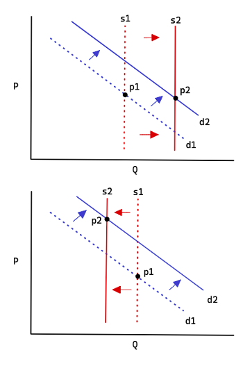
Conversely, the bottom graph attempts to depict the EIP-1559 mechanism. If we assume the shift from d1 to d2 is for transactions, which ultimately get burnt, then supply will shift from s1 to s2. You will notice that p2 is higher than where it would have been had supply remained at s1.
We can also demonstrate this behavior with a simple simulation. Starting with supply and demand functions of:
We assume \alpha_d follows a random walk around 100 with a standard deviation of .1. We also assume any \alpha_d in excess of 100 is for base fees and, as per EIP-1559, is burnt, shifting the supply curve to the left via a reduction in \alpha_s.
| n=1000 | cont. d | cont. s | \sigma_p |
|---|---|---|---|
| levels | 0.001 | 5.849 | 5.850 |
| changes | 0.067 | 0.024 | 0.091 |
| percent changes | 0.091 | 0.050 | 0.141 |
We see in the table above that a burn mechanism adds positively to the volatility of the equilibrium price since an increase in demand also decreases supply, both of which positively impact price.
Up until now, we have been using coincident levels and changes. However, using lags of \alpha_s may be more appropriate. For example, we may want changes in supply at time t-1 to be reflected at time t. Intuitively, supply may change to accommodate the next period’s demand. Alternatively, there may be a mechanism where supply expands or contracts at t+1 in response to changes at time t. Part of the problem is that we have not referenced time. Our data points could be individual blocks or some longer-term aggregate. If we look at block-level data, we would probably want to use leads or lags in changes of \alpha_s. Whereas over more extended periods, we would look at coincident changes.
What is important to recognize, however, as indicated by the contributions to changes in levels, is that changes in \alpha_s contribute meaningfully to the volatility of p_t in the long run. In our example, \alpha_d had a mean of 100, whereas \alpha_s continually decreased over time as a function of shifts in \alpha_d.
This analysis can many different paths. We have not considered changes in the slopes of the supply and demand curves, which may or may not even be linear. For example, as discussed in my previous piece, the demand curve for ETH may be negatively related to ETHUSD levels. We should look more holistically at the drivers of changes in supply and demand and their interactions, such as staking activity and risk premiums. Also, it would be illuminating to consider contributions to \sigma_p in different states of the world. For example, if we assume activity on Ethereum is procyclical, we expect demand for ETH to increase in good times and, thus, decrease the supply of ETH. Conversely, in bad times, the inflation from staking could approach the amount burnt, diminishing the contribution to ETHUSD volatility. In other words, there may be a compositional difference in contributions of supply and demand to upside and downside volatility in the ETHUSD rate.