A short follow-up to EIP-8411: what segmented payload diffusion is made of; the detailed technical report is here.
TL;DR
- We reran the EIP-8411 post’s main comparison under a second simulator, Shadow, over QUIC and over TCP, and the same code on the real Linux network stack.
- A-tuned, the design the post recommends, matches its earlier results within a few percent, and every segmented variant stays faster than the whole message in every configuration tested.
- The two simulators disagree on the whole message’s latency and on where variant C ranks; both trace to how a node’s uplink queue is modelled, fair queueing in the harness against first-come-first-served in Shadow. B’s completion tail is longer only under Shadow over QUIC.
- On one Linux machine, 100 processes on the kernel’s stack with the links shaped by its traffic control, A-tuned and C over QUIC land within the simulators’ own spread, and the whole message keeps the machine two to four times busier than the segmented variants.
- None of this tests the bandwidth model, a full client, or a node’s CPU cost on its own machine.
What the comparisons test
The earlier posts used one in-process harness: the real Prysm, go-libp2p and quic-go stacks over go-libp2p’s simulated network (simnet), under Go’s virtual clock. A result of 5 s to 0.7 s needs a check of how much depends on that harness.
Shadow runs one real process per node on real sockets and intercepts system calls. Its own TCP stack also lets us test TCP with yamux, which the harness cannot run. We reran the previous post’s Figure 1 with the same topology, links, latencies and seeds, ten seeds per point:
| comparison | what it tests |
|---|---|
| Published record versus harness twin | Whether code changes for Shadow compatibility changed the results; the twin uses the exact binary built for Shadow. |
| Harness twin versus Shadow QUIC | Whether the result survives a different simulator. |
| Shadow QUIC versus Shadow TCP | Whether the result depends on transport. |
Both simulators use cold connections with the libraries’ default windows, per-node uplink and downlink rates, fixed one-way latency per pair, and no cross-traffic. Both replace the operating system’s network stack, charge nothing for CPU time, and omit the full client. Their agreement increases confidence in the harness’s wiring and transport modelling; it adds no evidence about hashing cost or the bandwidth model.
The Linux run separately checks the kernel stack and the real clock, using one process per network namespace and virtual links from the same topology export. One machine cannot carry 500 nodes cleanly, so this check uses the 100-node cells in “What this says about reality” below.
A-tuned agrees; the baseline and alternatives vary
Segmentation lets a node forward parts before the whole payload arrives. A-tuned, the earlier post’s reference design, combines segmentation with selective pushes and disciplined requests. A carries segments on one gossipsub topic, B through the partial-message extension, and C on one topic per segment, each with and without a Reed–Solomon code (RS).
The cell uses 500 nodes and a 1 MiB payload, with home nodes at 50 Mbps up and 100 down. The builder publishes once; a node completes when it holds the whole payload. The 3 s budget is the time available to reach everyone.
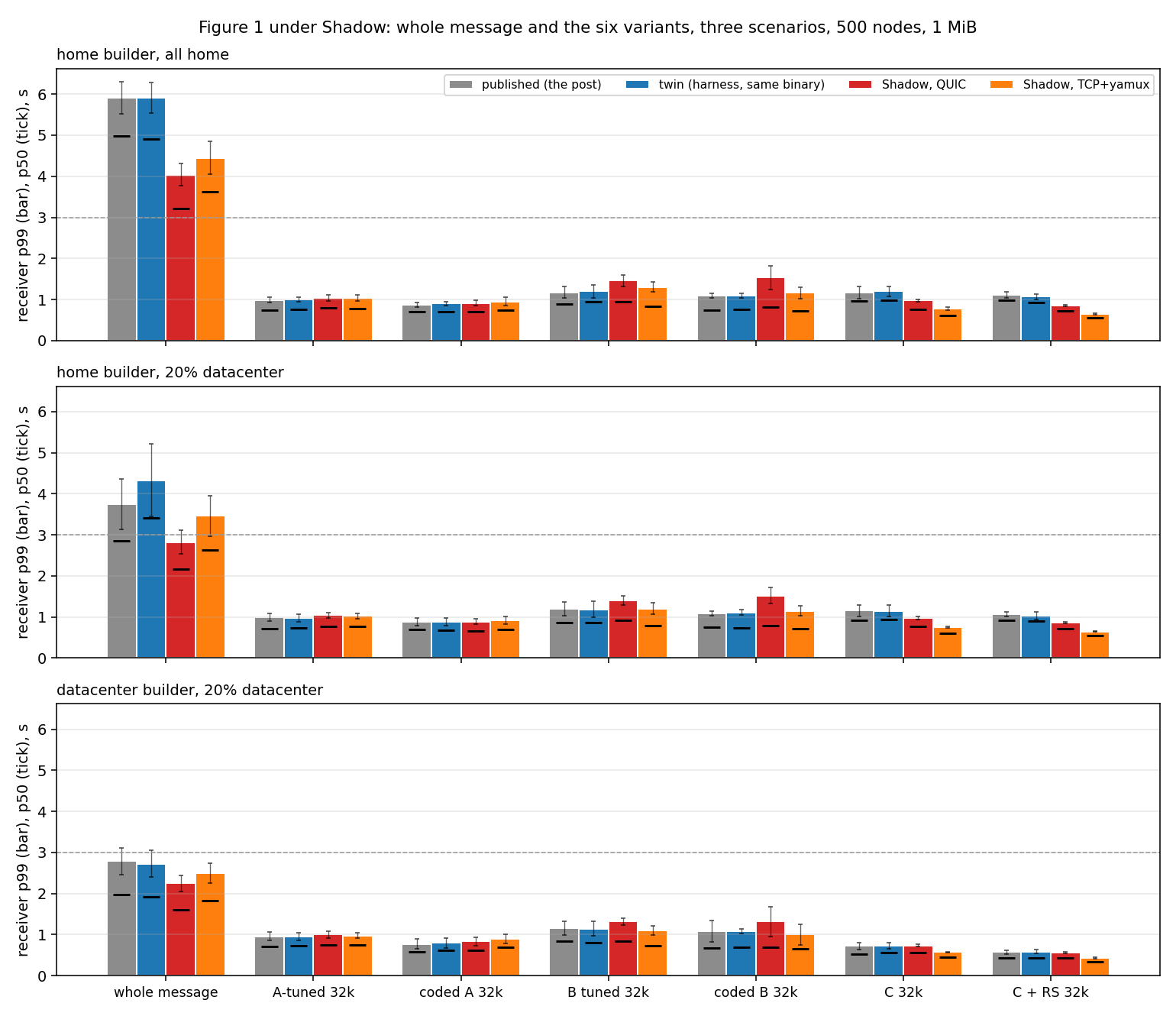
The post’s Figure 1, four columns per variant: the published record, its harness twin, Shadow over QUIC, Shadow over TCP. Bars: receiver p99; ticks: p50; both are medians across ten seeds, whiskers ±1 s.d.; dashed line: the 3 s budget. Three scenarios as in the post: home builder with all nodes at home, home builder with 20% datacenter nodes, datacenter builder with 20% datacenter nodes.
A-tuned reproduces within a few percent of its twin at both quantiles, in every scenario, on both transports. The twin matches the published record for every segmented variant; the whole message’s twin is 19% slower in the mixed scenario. Every segmented variant meets the 3 s budget on every side, and the whole message is always slowest.
The main difference is the uplink queue. The harness uses fair queueing (fq_codel); Shadow uses first-come-first-served (FIFO). When several copies compete for an uplink, fair queueing advances them together, so they all finish late. FIFO lets the first copy finish earlier, allowing its receiver to start the next hop while other copies wait. A has little queued at once; C’s concurrent meshes queue the whole payload’s worth in 32 KiB pieces, making its completion sensitive to that order.
These are configurations a node can encounter: a host or router can use fq_codel (RFC 8290), while an access device can use FIFO. Actual paths also contain routers, cross-traffic and other queue disciplines. PIE, for example, controls queue delay without sharing capacity between flows (RFC 8033); we have not measured it. The two results are not bounds on reality or evidence of which configuration is more common.
Three discrepancies remain:
-
The whole message is ~33% faster under Shadow (−34% against its twin at the median with a home builder, −16% with a datacenter builder). Switching Shadow to fair sharing over TCP reverses the advantage: the whole message becomes slower than on the harness. Queue order explains the advantage, but the switch does not quantitatively reproduce the harness.
-
C is ~20% faster under Shadow with a home builder, and faster again over TCP. Fair sharing removes about half of its TCP advantage. Shadow’s unpaced TCP benefits more from FIFO than paced QUIC does; a Linux TCP stack paces its sends too, so this extra benefit is mostly a simulation artifact, an inference from the kernel’s behaviour rather than a measurement. A residual of about a tenth on both transports, with more duplicates under Shadow, remains unexplained. A is insensitive to the queue in every configuration measured, while C moves from the slowest segmented variant on the harness to among the fastest under Shadow. The report gives the socket and pacing mechanics.
-
B’s tail is longer only under Shadow QUIC (coded B’s p99 is +40% against its twin with a home builder; medians agree within 7%; TCP tails match). B claims each part from one peer and waits, exposing slow service that A’s redundant pushes can mask. Capping the shared UDP send buffer from 7 MB to 64 KB removes about a third of the excess tail at one seed. The remaining tail is unexplained.
For the whole-message baseline, the harness and Shadow give 4.9 s and 3.2 s medians at 500 nodes and 1 MiB with a home builder. Both miss the budget; A-tuned’s improvements are 6.5× and 4.1×. The earlier posts report the harness’s number.
What this says about reality
The Linux check adds the kernel network stack and CPU time that both simulators omit. It uses the same node binary, rates and one-way delays, either uplink queue, and a wall-clock publish. The largest cell one 40-thread machine carries cleanly for the segmented variants is 100 nodes at degree 70. Above that, host saturation dominates delivery time.
At 100 nodes and 1 MiB with home link bandwidth, the tables give medians across seeds of receivers’ p50 / p99 completion time in seconds and the real-stack difference from the paired simulator. Host CPU is the mean over all 40 threads during the 10 s after publish. First, FIFO against Shadow:
| variant | transport | Shadow (s) | real stack (s) | real stack vs Shadow (%) | host CPU (%) |
|---|---|---|---|---|---|
| whole message | QUIC | 2.20 / 2.95 | 3.61 / 4.78 | +68% / +58% | 35 |
| A-tuned | QUIC | 0.76 / 1.00 | 0.78 / 1.07 | +4% / +9% | 8 |
| C | QUIC | 0.71 / 0.93 | 0.85 / 1.06 | +18% / +15% | 14 |
| whole message | TCP | 2.72 / 3.74 | 3.32 / 4.37 | +23% / +18% | 23 |
| A-tuned | TCP | 0.75 / 0.97 | 0.97 / 1.31 | +27% / +37% | 7 |
| C | TCP | 0.56 / 0.73 | 0.93 / 1.18 | +66% / +61% | 14 |
Then fq_codel against the harness, which runs QUIC only:
| variant | transport | harness (s) | real stack (s) | real stack vs harness (%) |
|---|---|---|---|---|
| whole message | QUIC | 3.49 / 4.76 | 4.22 / 5.53 | +25% / +18% |
| A-tuned | QUIC | 0.68 / 0.94 | 0.78 / 1.09 | +14% / +17% |
| C | QUIC | 0.88 / 1.10 | 0.89 / 1.11 | −1% / −1% |
| whole message | TCP | – | 4.40 / 5.60 | – |
| A-tuned | TCP | – | 0.93 / 1.33 | – |
| C | TCP | – | 0.97 / 1.22 | – |
With each simulator paired to the queue it models, segmented QUIC is within −1 to +18% of the simulators on the real stack, with the same bytes and meshes, within the simulators’ own spread on these cells. The larger TCP gaps compare Linux TCP with Shadow’s implementation and therefore bear on Shadow’s TCP fidelity.
The whole message is slower than both simulators. Over QUIC, host CPU contributes to that result: spreading one 1 MiB message keeps the machine two to four times busier than spreading segments. At 250 nodes it stays busy through most of an 8 s delivery, while the segmented variants saturate it for about a second. This is evidence from one shared host and kernel; it does not measure a node on its own machine. The report’s section 10 gives the transport, queue and saturation details.
Segmentation moves the median from seconds to under a second on both simulators and both transports; the real-stack segmented results fall within the simulators’ own spread. Segmentation’s advantage survives these cross-checks; the exact speedup and ranking of alternatives depend on the network model.
The technical report contains the method, size sweeps, sensitivity tests and open questions. The earlier harness is in segstudy; eth-networking-lab prepares Shadow cells and pairs their records with the harness.
Note: the code behind this post, the node, the simulator tooling and the patched Shadow, is pinned at tag shadow-crosscheck of eth-networking-studies, with the commands to run a cell in its README. The clean prototype of variant A is still the variant-a branch of Prysm.