Folding over quartic extensions in 2N-4 multiplications, and why row-based commitment layers can’t keep up
TL;DR
We give an exact algebraic backend for sumcheck-style folding over a quartic extension E/F. Using a moving power basis \{1, r_i, r_i^2, r_i^3\} that tracks the reciprocal orbit, the fold engine performs exactly 2N - 4 base-field multiplications on F-valued leaves — a 5× reduction over the direct fixed-basis baseline. The entire seed-specialized evaluator T_{\tau,n}: F^N \to F^4 is described by a reduced public descriptor of 4(n-1) field words, compared to the 4N words required by explicit row vectors. However, any downstream commitment layer that accepts only explicit rows cannot consume this compression and must materialize the full 4N-word representation.
Motivation
Sumcheck-style folding protocols describe their round-by-round updates at a schematic level. For quadratic extensions this is harmless — the local fold is a textbook identity. But starting at degree 4, three things become nontrivial simultaneously: the moving-basis transport after each reciprocal step, the coefficient update for the round minimal polynomial, and the exact multiplication count of the resulting engine.
No prior work isolates all three in closed form for a fixed extension degree. This matters for downstream layers: without an exact algebraic specification, commitment and opening protocols must either re-derive the round structure internally or fall back to generic row-vector interfaces that forfeit the logarithmic-size seed specialization.
This note fills that gap for the quartic case [E:F] = 4 with an alternating 0/1 schedule, and records the interface consequence that explicit-row consumption destroys the compression.
Results: fold engine performance
Fix F = \mathbb{F}_q with \text{char}(F) > 3, E = \mathbb{F}_{q^4}, and N = 2^n. The following table compares the specialized moving-basis fold against the direct fixed-basis baseline, both measured on the BN254 scalar field.
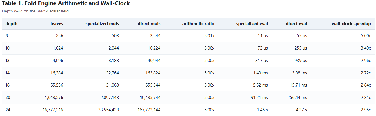
Every entry in the specialized muls column equals exactly 2N - 4, confirming the theoretical count. The multiplication ratio converges to 5.00× across all tested depths, matching the asymptotic prediction (m_{F,\text{pub}} + m_{E,\text{pub}})/4. Wall-clock speedups range from 2.72× to 5.00×; the gap from the arithmetic ratio reflects memory-hierarchy effects at larger N.
How it works
The algebraic engine has three layers. We sketch only the essential identities; full proofs are in the note.
1. Reciprocal orbit
Fix a seed \tau \in E with F(\tau) = E. Define the public challenge orbit by
$$r_1 = \tau, \qquad r_{i+1} = \frac{1}{r_i - c_i}, \qquad c_i = \begin{cases} 0, & i \text{ odd}, \ 1, & i \text{ even}. \end{cases}$$
Every orbit point satisfies F(r_i) = E, so \{1, r_i, r_i^2, r_i^3\} is an F-basis of E at every round. The live state of the fold engine is always a four-word vector (a_0, a_1, a_2, a_3) \in F^4, interpreted through a shared denominator as an element of E.
2. Local fold (Step A)
At round i, an adjacent pair of states (s_0, s_1) is folded by
$$u = s_0 + S_{\mu_i}(s_1 - s_0),$$
where
$$S_{\mu} = \begin{pmatrix} 0 & 0 & 0 & \mu_0 \ 1 & 0 & 0 & \mu_1 \ 0 & 1 & 0 & \mu_2 \ 0 & 0 & 1 & \mu_3 \end{pmatrix}$$
and \mu_i = (\mu_{i,0}, \mu_{i,1}, \mu_{i,2}, \mu_{i,3}) are the coefficients of the minimal polynomial of r_i. The key structural fact: on F-valued leaves, the difference vector s_1 - s_0 concentrates all seed dependence into a single scalar \delta_3. Step A therefore costs exactly 4 multiplications per surviving pair — one for each \mu_j \delta_3.
3. Chart transport
After Step A, the state must be re-expressed in the next round’s basis. This is the transport map R_{c_i}:
-
Odd rounds (c_i = 0): R_0(u_0, u_1, u_2, u_3) = (u_3, u_2, u_1, u_0). A coordinate reversal — zero multiplications.
-
Even rounds (c_i = 1): R_1 involves additions and multiplications by the public constants 2 and 3, which are realized by add-chains — zero multiplications under the canonical cost model.
The total count over all rounds is therefore: round 1 contributes 0 (scalar inputs), and each subsequent pair contributes exactly 4 multiplications from Step A. Summing:
$$M_{\text{canon}}(N) = 4 \cdot \left(\frac{N}{2} - 1\right) = 2N - 4.$$
Worked example: N = 4
The case N = 4 is the smallest nontrivial instance. Let x = (x_0, x_1, x_2, x_3) \in F^4 and \mu_2 = (\mu_{2,0}, \mu_{2,1}, \mu_{2,2}, \mu_{2,3}). The full evaluator matrix is:
$$T_{\tau,2}(x) = \begin{pmatrix} 2-\mu_{2,3} & -1 & \mu_{2,3}-1 & 1 \ 5-\mu_{2,2}-3\mu_{2,3} & -2 & \mu_{2,2}+3\mu_{2,3}-3 & 3 \ 4-\mu_{2,1}-2\mu_{2,2}-3\mu_{2,3} & -1 & \mu_{2,1}+2\mu_{2,2}+3\mu_{2,3}-3 & 3 \ 1-\sum_{j}\mu_{2,j} & 0 & \sum_{j}\mu_{2,j}-1 & 1 \end{pmatrix} \begin{pmatrix} x_0 \ x_1 \ x_2 \ x_3 \end{pmatrix}.$$
The four rows are the explicit row vectors \lambda_{\tau,2}^{(0)}, \dots, \lambda_{\tau,2}^{(3)}. The multiplication count is M_{\text{canon}}(4) = 4 = 2 \cdot 4 - 4, matching the general formula.
Note that \mu_1 does not appear: the first round on scalar leaves is seed-independent, so the reduced descriptor for n = 2 contains only \mu_2 — exactly 4(n-1) = 4 field words.
The interface consequence
The evaluator T_{\tau,n} is a public F-linear map from F^N to F^4. A downstream commitment or opening layer can interact with this object in two ways:
-
Consume the structured descriptor (\mu_2, \dots, \mu_n) directly — 4(n-1) field words.
-
Materialize the four explicit row vectors \lambda_{\tau,n}^{(k)} \in F^N — 4N field words.
Option 2 is forced whenever the commitment API accepts only Vec<F> rows. The next table shows what this costs in practice.

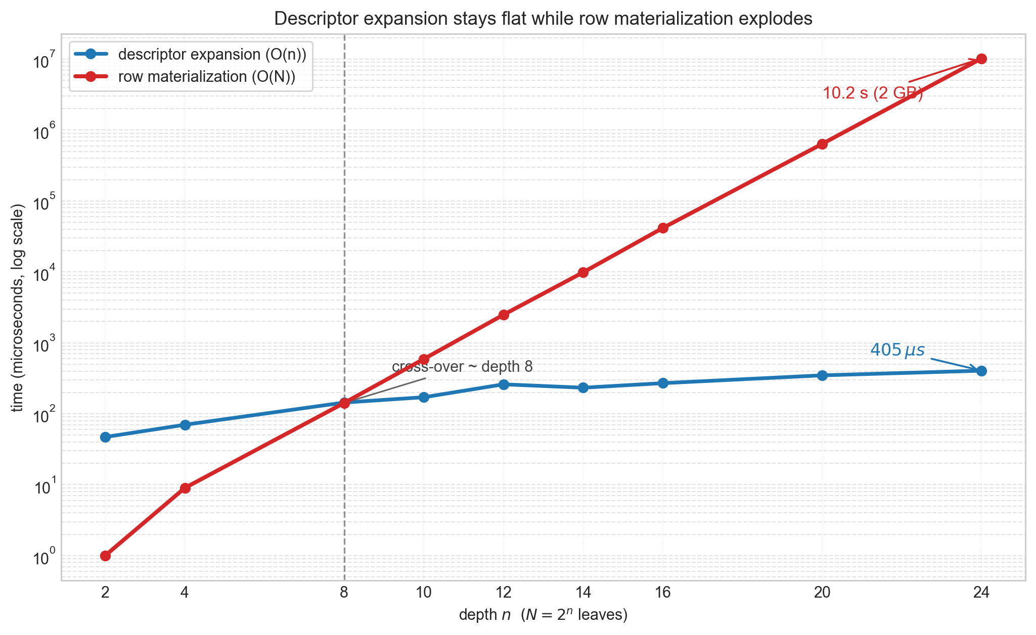
The pattern is clear. Descriptor expansion runs in O(n) time and stays under 500 μs even at depth 24. Row materialization runs in O(N) time: at depth 20, it already takes 637 ms and produces 128 MB of payload; at depth 24, it takes 10.2 seconds and produces 2 GB.
This is not a hardness claim — the rows can be computed in linear time from the structured descriptor. It is an interface claim: the moment a downstream layer chooses a row-only API, the logarithmic seed specialization is destroyed. A 4(n-1)-word descriptor that fully determines the evaluator must be expanded into 4N explicit coefficients, converting a 92-word object into a 2 GB payload at N = 2^{24}.
Any downstream layer that wants to preserve the O(n)-word specialization must consume the structured reciprocal descriptor itself — or something equivalent to it — rather than only explicit row vectors.
Soundness note
The note also records a minimal information-theoretic soundness result. The deterministic orbit transcript — where the public orbit points r_1, \dots, r_n are reused as sumcheck challenges — is perfectly unsound: a cheating prover can force acceptance with probability 1 for any false claim. This holds because r_i \notin \{0, 1\} gives the prover enough degrees of freedom at every round.
The fix is standard: commit the claimed output y \in F^4 before seeing a fresh random scalarization vector \rho, then run sumcheck with fresh independent verifier challenges in F. In an oracle model where the verifier has exact access to the input’s multilinear extension at the final sampled point, a false claim y \neq T_{\tau,n}(x) is accepted with probability at most (2n+1)/q.
Full proof: Section B of the note.
Open questions
-
Structured commitment consumption. Can practical commitment schemes (KZG-based, lattice-based, or IPA-based) consume the 4(n-1)-word structured descriptor directly, without materializing explicit rows?
-
Higher-degree generalization. The quartic case is isolated here because all local identities fit in closed form. For [E:F] > 4, how does the transport complexity grow, and does the moving-basis advantage persist?
-
End-to-end impact. The benchmarks above measure kernel-level arithmetic. Is much of the 5× multiplication reduction expected to survive once commitment, opening, and Fiat–Shamir overhead are included?