What happens to the fee market when Glamsterdam changes transaction gas costs and the gas limit rises from 60M to 200M? More capacity should ease pressure on fees, but cheaper gas also attracts demand. The outcome depends on how much demand arrives and how strongly users respond to the change in price. In addition, the gas limit grows gradually, so the fee market has time to adjust.
In this report, we simulate the first 7,200 blocks, or roughly one day, under twelve demand scenarios. The Glamsterdam gas schedule applies from the first block. The limit takes about four hours to reach 200M, leaving roughly twenty hours to observe how fees and block utilisation settle.
Under the demand assumptions tested here, the day has a clear sequence: an initial fee spike, a decline as capacity expands and demand responds, and then an adjustment around the new 100M target. The size of the spike depends heavily on how the demand scenario.
After this adjustment phase, nine of the twelve demand scenarios have median utilisation near the EIP-1559 target, with median base fees ranging from 0.0002 to 0.3928 gwei. The other three remain below target even with an almost negligible base fee.
How is the simulation set up?
We start with roughly 21 days of historical mainnet transactions, replayed upstream with the Glamsterdam gas schedule implemented in an instrumented reth fork. This replay records how much gas each transaction uses under the new rules. Those measurements become fixed inputs to the simulation: sampling a transaction again does not re-execute it.
The simulation begins immediately after the fork, with the new gas schedule already active and the gas limit still at 60M. From the next block onwards, the limit increases by approximately 1/1024 of its previous value per block, until it reaches 200M at block 1,234, about four hours later.
At each simulated block, we repeat three steps:
- Sample arrivals. A demand model determines how much gas arrives: higher prices reduce demand, and lower prices increase it. We sample historical transactions to meet that quantity and add them to the mempool alongside transactions waiting from earlier blocks.
- Build the block. We select transactions that can pay the current base fee, ordered by effective tip. Each transaction is included if it fits within the remaining capacity. If it does not fit, we skip it and continue. Transactions left out remain in the mempool.
- Update the fee for the next block. We apply the EIP-1559 rule using this block’s utilisation. The base fee rises when utilisation exceeds the 50% target and falls when utilisation is below it. The block’s base fee and realised tips also update the price signal that determines subsequent demand.
This creates a feedback loop: fees change arrivals, arrivals change block utilisation, and utilisation changes the next base fee. As the limit grows, the fee target rises from 30M to 100M gas per block.
Additionally, block capacity follows two new accounting rules:
- Execution gas and state-creation gas must each fit within the limit, and utilisation is the larger of the two divided by the limit. This is introduced by EIP-8037.
- Block capacity is measured before refunds (i.e., gas refunds do not count towards the block limit, per EIP-7778).
What demand are we assuming?
The historical transactions supply the mix of work. The demand model determines how much of that work arrives at each block. It measures quantity as execution gas plus state gas, rather than transaction count. This demand measure differs from block utilisation, which uses the larger dimension.
Demand responds to a smoothed effective price (base fee plus tip). We compare that price with a fixed reference price from the historical trace. When the simulated price falls below the reference, the model samples more demand. When it rises above it, the model samples less. Including tips matters when the base fee becomes negligible, because users still pay to have transactions included. An exponential moving average with a 200-block span makes the response gradual.
We also vary two assumptions:
- Demand level: 1x, 1.5x, 2x or 2.5x. This sets the quantity arriving at the reference price. At 1x, it is one historical average block’s worth of gas per simulated block, while at 2x, it is twice that amount. Actual arrivals then rise or fall with the simulated price, so a 2x scenario does not keep arrivals fixed at twice the historical quantity.
- Price elasticity: 0.1, 0.2 or 0.3. This sets the strength of the response. Halving the effective price increases demand by roughly 7%, 15% or 23%, respectively. A larger elasticity therefore brings more demand back when fees fall, and reduces it more when fees rise. These values follow a previous empirical analysis.
The price signal starts at the historical reference, so initial demand is exactly the chosen level. That level applies in full from the first block, while the gas limit grows gradually. This timing is important for interpreting the early fee spike.
We simulate 50 paths for each of the twelve combinations. The next section shows the initial 3,000 blocks, or roughly ten hours, covering the ramp and the early settling period. The section after that shows the full 7,200-block day. The lines in the charts are means across paths and shaded bands show their 10th–90th percentile. The full-day chart uses 24-block averages within each path.
The first several hours: fees rise before capacity catches up
The transition starts with demand arriving against a 60M limit. The higher-demand scenarios initially fill blocks close to that limit, while even the 1x scenario starts above the 30M gas target (due to the increase in gas costs from repricings). The following plot shows this trend. The horizontal dashed line marks the 50% utilisation target, while the vertical dashed line marks the end of the ramp at block 1,234.
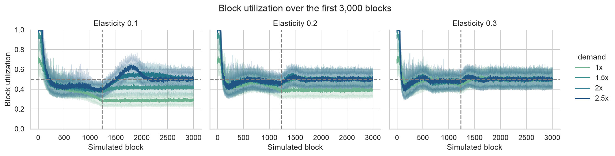
With utilisation above target, EIP-1559 raises the base fee. Demand then falls as the smoothed effective price catches up. Meanwhile, the growing gas limit creates more room in each block. Together, these effects bring utilisation below target, causing the base fee to fall again.
Higher elasticities produce an earlier, smaller fee peak. At the lowest elasticity, demand is less sensitive to price, so the base fee rises much higher before falling again. The base-fee axis is logarithmic, so the spike spans several orders of magnitude.
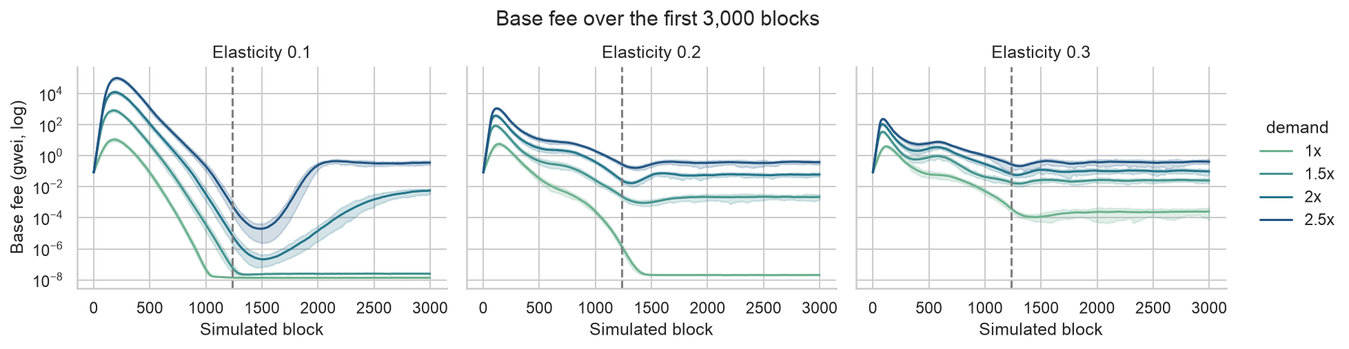
The spike reflects the starting assumptions: full demand from block 0, a 60M initial limit, and a price signal that adjusts gradually from the historical reference. Together, these allow demand to stay high while the base fee rises sharply.
The spike therefore illustrates what can happen when demand arrives faster than capacity and reacts with a delay. Its magnitude should not be read as a forecast. This sweep does not test demand arriving gradually alongside the capacity increase, or alternative response delays.
In all scenarios, this adjustment phase occurs in the first several hours, with weaker price responses taking longer to recover. Fees and utilisation have approximately stabilised in all scenarios by block 3,000, about ten hours into the simulation. We use blocks 3,000–7,199, the remaining fourteen hours, for all settled-period medians below.
The rest of the day: two outcomes emerge
Once the limit reaches 200M and fees stabilise, the scenarios separate into two groups: those that attract enough demand to approach the 100M fee target, and those that remain below it even as the base fee becomes negligible.
Under this transaction mix, reaching the 100M fee target requires roughly 2.54 times the reference demand quantity. The horizontal dashed line in the plot below marks that multiplier. The plot follows demand through the full day, from its initial fall to its recovery as prices ease.
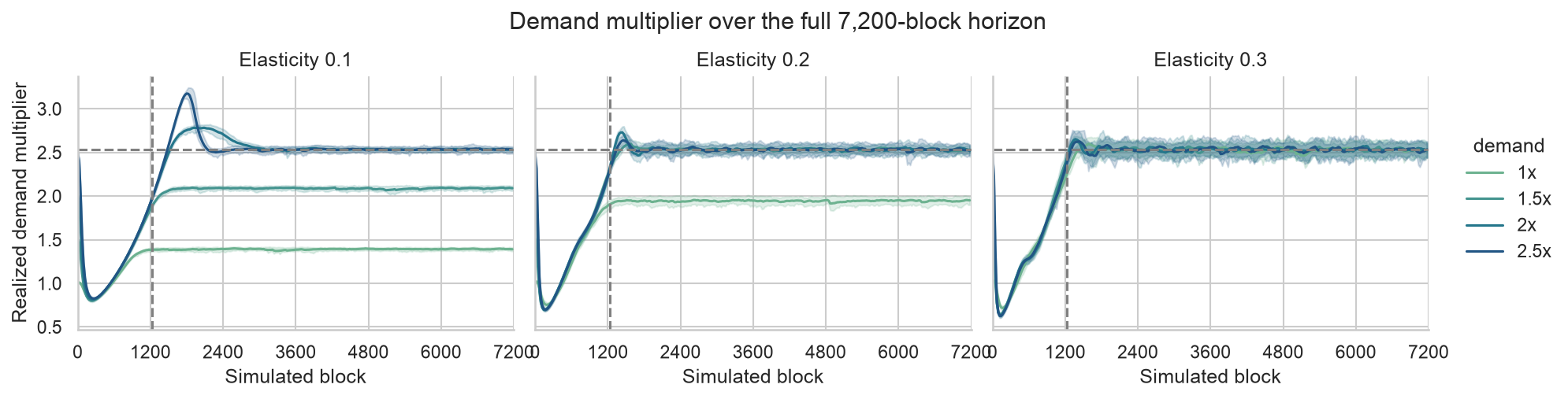
Nine scenarios settle near the dashed line, while three level off below it. These are the two outcomes described below.
1. Enough demand to reach the fee target
Nine of the twelve scenarios have a settled-period median utilisation of roughly 50%. The feedback explains why these scenarios look similar on the utilisation chart. If arrivals remain above target, the base fee rises and reduces demand. If arrivals fall below target, the fee falls and attracts more demand. This brings the scenarios towards the same quantity, despite starting from different demand assumptions.
2. Too little demand, even with a negligible base fee
The remaining three scenarios cannot attract enough demand to reach the 100M target:
| Demand scenario | Settled-period median utilisation | Gas used per block |
|---|---|---|
| 1x, elasticity 0.1 | 28.3% | 56.5M |
| 1x, elasticity 0.2 | 38.7% | 77.4M |
| 1.5x, elasticity 0.1 | 41.4% | 82.8M |
Here the base fee falls to a few tens of wei and stays negligible. Further reductions barely change the effective price because tips dominate: in the 1x, elasticity 0.1 scenario, the gas-weighted average tip per block has a median of about 0.025 gwei. With a weak price response, making the base-fee component nearly free does not bring enough additional demand to reach target.
This is the main low-demand outcome of the simulation: some of the new capacity remains unused, and tips account for almost all of the gas price paid by users.
Similar utilisation can come with very different fees
Reaching the same block utilisation does not mean paying the same price. Among the nine scenarios near 50% utilisation, different demand levels and price elasticities sustain very different base fees.
The chart below compares median base fees over blocks 3,000–7,199, after fees and utilisation have approximately stabilised in all scenarios. The dashed line marks the starting fee of about 0.085 gwei. As we can see, a larger limit does not guarantee a lower base fee if enough demand arrives.
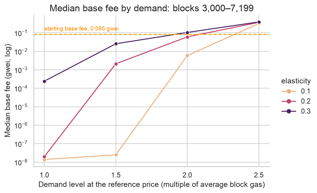
The table gives the corresponding median base fees in gwei, based on 20,000 individual blocks sampled from blocks 3,000–7,199 across the 50 paths per scenario.
| Demand level | Elasticity 0.1 | Elasticity 0.2 | Elasticity 0.3 |
|---|---|---|---|
| 1x | <0.0001 | <0.0001 | 0.0002 |
| 1.5x | <0.0001 | 0.0021 | 0.0258 |
| 2x | 0.0059 | 0.0609 | 0.1058 |
| 2.5x | 0.3199 | 0.3722 | 0.3928 |
At 2x demand, for example, all three elasticities produce roughly 50% utilisation, but the median base fee ranges from about 0.006 to 0.106 gwei. When demand responds more strongly to cheaper gas, a smaller price reduction is enough to attract the quantity needed for the target. The fee therefore stays higher.
At 2.5x demand, the scenarios already start close to the quantity needed at 200M, so less price adjustment is required. Their settled-period median fees are closer together, around 0.32–0.39 gwei. That narrowing does not mean elasticity is unimportant: it has a large effect on the early fee spike and on the lower-demand outcomes.
Assumptions and limitations
- The transaction mix is fixed. Transactions retain their upstream gas measurements when sampled or reordered. The simulator does not re-execute them against the resulting state, enforce nonces, balances, state dependencies or bundles, or predict how applications adapt to new gas costs. The source contains included transactions, so 1x is an observed-demand reference rather than a measurement of all potential demand.
- Demand responds only to price. One aggregate elasticity covers both gas dimensions and cannot represent substitution between them. Estimates based on historical daily data and base fees are applied to block-level effective prices and much lower fees. Confirmation delays do not deter arrivals, and adapted fee caps do not model users rebidding.
- Capacity uses measured gas. The model does not reserve space using transaction gas limits. Execution gas is usually the larger dimension, but state gas is larger in about 19–21% of blocks across scenarios and sometimes nearly fills the limit during the transition. About 85% of the trace’s state gas comes from transactions that would need higher signed gas limits to succeed under the new schedule, an adaptation assumed in these inputs.
- The transition and sampling choices are untested sensitivities. Demand applies immediately, the price signal is smoothed, and transaction mixes are drawn independently from pools of 16 neighbouring source cohorts. Historical demand persistence is not preserved. This sweep does not vary those choices, and the one-day horizon limits conclusions about later behaviour. Numerical bounds on price response and base fee are model safeguards; neither the base-fee ceiling nor the demand-response bounds are hit in this run.
Reproducing the analysis
The report uses run 20260907T122124Z, drawing on source blocks 25,168,786–25,319,985, a span of roughly 21 days. It contains twelve scenarios with 50 paths each, all simulated for 7,200 blocks. The demand reference is the trace’s gas-weighted effective price of 1.0130 gwei, paired with average demand of 61.33M gas on the execution + state basis. That sum measures demand; block utilisation uses the larger dimension, so the two quantities should not be compared directly.
The price-response factor is bounded between 0.05 and 20 before multiplication by the demand level. Complete configuration, accounting rules and output definitions are in the methodology, with analysis and supporting diagnostics in the notebook.