LeanDA: Design and Benchmark

LongMeng · August 6, 2026, 2:32pm

Authors. Long Meng, Benedikt Wagner, George Kadianakis, Francesco Risitano

Thanks to Tom Wambsgans, Thomas Coratger, Arantxa Zapico, and others for insightful discussions.

1. Motivation

Ethereum uses data availability sampling (DAS) to let validators check the availability of large blob data by sampling a small number of random positions from an erasure-coded object, rather than downloading the whole payload. As Ethereum moves toward post-quantum security, the current DAS protocol based on KZG polynomial commitments needs post-quantum alternatives.

This post first shows an encode + prove type of PQ-DAS construction instantiated with Reed-Solomon code, hash commitments, and the LeanVM proof system, and then show benchmarks for various input parameters and output metrics. The code for the up-to-date implementation is at: LongMeng-Crypto/PQ-DAS. A companion document containing the benchmark and security results is available in Supplementary.md.

2. Encode + Prove DAS: Workflow

In general, a DAS protocol consists of a set of users, a block builder, and a set of verifiers. The benchmarked DAS protocol in this report is the Encode + Prove paradigm from the solution space of the DAS foundations, Section 7. In this class, the builder encodes the data with an erasure code, commits to the codewords by using a vector commitment scheme, and proves that the committed object is a valid codeword by using a SNARK proof system. Sampling opens authenticated positions of the codeword symbols, while reconstruction uses accepted samples as erasure-code evaluations.

Abstractly, the workflow of such a DAS protocol is as follows:

Initialization: All users send their data to the builder.
Commit: The builder receives data from the users, first encodes them and commits to the codeword, then it generates a SNARK proof for proving that the data are encoded into the codewords, and the codewords are commited as the commitment. Finally, the builder uploads the commitment, the SNARK proof, and the codewords including commitment openings for all symbols to the network.
Download Commitment: Each verifier downloads the full commitment and SNARK proof from the network. Each verifier checks if the SNARK proof verifies with respect to the commitment. If not, they reject immediately.
Sampling and Verification: Each verifier samples a random set of indices and tries to download the corresponding codeword symbols and their openings from the network. Each verifier checks if the received openings are valid against the commitment. If not, they reject. If they are all valid, they accept.

Intuitively, if any party collects enough symbols that have been verified, the original data can be reconstructed and missing symbols can be reinserted into the network, to help other verifiers to eventually accept.

Informally, a DAS scheme should satisfy the following security properties: completeness, (subset-)soundness, consistency, and repairability. For the formal definition of the DAS syntax and these properties, we refer to the DAS foundations.

Other schemes. In this post, we do not focus on other post-quantum alternatives such as FRIDA and ZODA. This is because they do not satisfy a crucial property called repairability, which is achieved by the current KZG solution and implicitly assumed throughout the protocol. Informally, this property ensures that reconstructed symbols can be reinserted into the network and verify with respect to the (potentially maliciously generated) commitment. This ensures that parties will eventually agree on whether data is available or not. Without this property, one would have to significantly adapt the surrounding protocol.

3. Concrete Construction

After introducing the overall workflow, we will now make more precise how the considered constructions work. In particular, we will define how the commitment is computed and which codes are used. While doing so, we also introduce the parameters that we will vary in our benchmarks.

The following image illustrates the workflow:

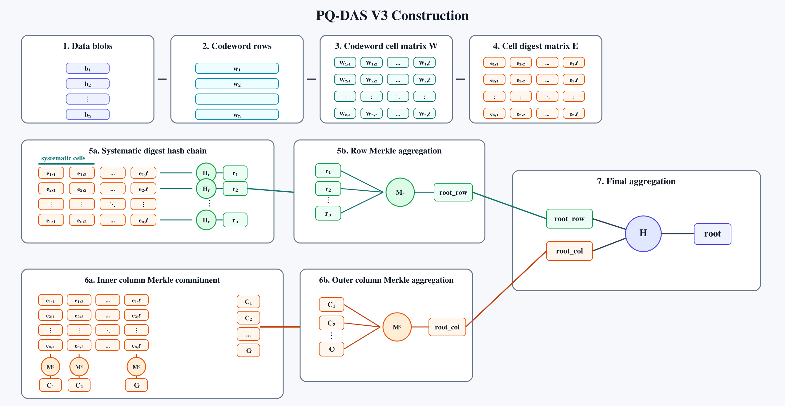
For the construction, we use the Poseidon hash function, denoted as \mathsf{H}; we fix the erasure code as Reed-Solomon (RS) code over the field \mathbb{F}, which is the KoalaBear quintic extension field. For the evaluation domain, we use the roots of unity in the KoalaBear base field, so that encoding is given by an FFT;

We choose Merkle tree commitment as the vector commitment scheme; and we use LeanVM as the SNARK proof system. Below, we also describe which relation is proven using LeanVM.

Very roughly, the construction works by arranging the data into rows of a matrix as in PeerDAS and extending each row via the Reed-Solomon code. Instead of KZG commitments, we use Merkle roots, and we additionally add a SNARK as explained above.

More precisely, we set the row length k, the encoded row length m = 2k (meaning rate \rho = 1/2), the cell size c, the number of cells per row \ell=m/c, and the reconstruction threshold t=\lceil k/c\rceil. Each data object is parsed into n rows (each row is called a blob today), each row is encoded as one Reed-Solomon codeword, and the first k symbols are systematic payload symbols. With these paramerers, the protocol workflow is described as follows:

Initialization: All users send their data to the builder.
Commit: The builder operates following steps:
Encodes each each blob of data into a RS codeword. We denote w_i as the i-th row of codeword.
Arranges all codewords into a n\times m matrix, where each row is one codeword. Then the codeword on each row i \in [1, n] is split into \ell consecutive cells W_{i,j}\quad (j \in [1, \ell]), where each cell contains c field elements. Every cell is hashed into a digest e_{i,j}=\mathsf{H}(W_{i,j}).
For every row i, the first t cell digests, which cover the systematic payload cells, are hashed into a row digest r_i=\mathsf{H}(e_{i,1},\ldots,e_{i,t}). The row digests are then committed via a Merkle tree into \mathsf{root}_{\mathsf{row}}. This row commitment gives a compact binding to each row’s systematic data.
For every cell column j \in [1, \ldots, \ell], the digests (e_{1,j},\ldots,e_{n,j}) are aggregated through a Merkle tree into a column root C_j. The column roots (C_1,\ldots,C_{\ell}) are then further aggregated through a Merkle tree into \mathsf{root}_{\mathsf{col}}.
The row root \mathsf{root}_{\mathsf{row}} and column root are further hashed together to form the commitment \mathsf{root}=\mathsf{H}(\mathsf{root}_{\mathsf{row}},\mathsf{root}_{\mathsf{col}}).
Computes the public Reed-Solomon membership check vector L from public parameters and \mathsf{root}. The details of how to compute L via Fiat-Shamir can be referred to the next section “RS Membership Check Instantiations”.
The LeanVM proof \pi binds these commitments to valid Reed-Solomon codewords. In particular, \pi \leftarrow \mathsf{LeanVM}.\mathsf{Prove}(\mathsf{pp}_{\mathsf{STARK}}, \mathsf{stmt}, \mathsf{witn}, \mathcal{R}).

The public statement, witness, and proved relation are defined as follows:

\begin{aligned} \mathcal{R} = \{(\mathsf{stmt},\mathsf{witn}) \;:\;& \mathsf{stmt} = (\{r_i\}_{i \in [1, n]}, L, \mathsf{root}), \\ & \ \mathsf{witn}= \{W_{i, j}\}_{i \in [1, n], j \in [1, \ell]}, \\ & \forall i\in[1,n],j\in[1,\ell],\; e_{i,j}=\mathsf{H}(W_{i,j}),\\ & \forall i\in[1,n],\; r_i=\mathsf{H}(e_{i,1},\ldots,e_{i,t}),\\ & \mathsf{root}_{\mathsf{row}}=\mathsf{Merkle.Com}(r_1,\ldots, r_n), \\ & \forall j\in[1,\ell],\; C_j=\mathsf{Merkle.Com}(e_{1,j}, ..., e_{n,j}),\\ & \mathsf{root}_{\mathsf{col}}=\mathsf{Merkle.Com}(C_1, ..., C_{\ell}),\\ & \forall i\in[1,n],\; \langle L, w_i\rangle=0 \}, \\ & \mathsf{root} = \mathsf{H}(\mathsf{root}_{\mathsf{row}}, \mathsf{root}_{\mathsf{col}}). \end{aligned}

After generating the proof, the builder generates the Merkle authentication paths for the column cells W_{1,j},\ldots,W_{n,j} for every j \in [1,\ell]. It then uploads all codeword cells W_{i,j}, the row hashes r_i\quad(i \in [1,n]), the column root \mathsf{root}_{\mathsf{col}}, the LeanVM proof \pi, and the Merkle openings for all column cells.

Download Commitment: Each verifier downloads the row hashes r_i\quad(i \in [1,n]), the column root \mathsf{root}_{\mathsf{col}}, the leanVM proof \pi. Each verifier computes \mathsf{root}_{\mathsf{row}} from r_i\quad(i \in [1,n]) and computes \mathsf{root} = \mathsf{H}(\mathsf{root}_{\mathsf{row}}, \mathsf{root}_{\mathsf{col}}), recomputes the vector L from public parameters and \mathsf{root}, checks if \pi verifies with respect to \mathsf{root}. If not, they reject immediately.
Sampling and Verification: A verifier samples a set Q of cell-column indices, queries the network and downloads the sampled columns W_{1,j},\ldots,W_{n,j} for j \in Q, and their Merkle tree paths to the final \mathsf{root}. Each verifier checks if Merkle paths are valid against \mathsf{root}. If not, they reject. If they are all valid, they accept.

4. RS Membership Check Instantiations

In the relation we prove, we ultimately want to check that each row of codeword w_i is a valid RS codeword. We implement this via a simple inner product with a random vector L.

There are different ways for instantiating this check. We investigate three approaches, which are respectively the parity check, the generic barycentric check, and a special form of barycentric check for when the RS code rate \rho = {1}/{2}. The details of all these approaches are at RS membership check.

The computational overhead for these three approaches is very close. For a length-m codeword and n rows, computing the public vector L outside the proof costs \mathcal{O}(m) field operations after Fiat-Shamir. Inside the proof, the RS membership relation is one length-m inner product per row, so the total in-proof cost is \mathcal{O}(nm) field operations.

In our implementation, we choose the special barycentric check because our benchmarked RS code has rate \rho=1/2, so the codeword can be split into even and odd evaluations and membership reduces to the single identity A_i(p)=B_i(p/\omega). Compared with the parity-check method, it avoids constructing a random linear combination over all high-degree coefficients; compared with the general barycentric check, it avoids evaluating arbitrary Lagrange bases over a chosen systematic split. Thus it has slightly cheaper computations and hence cheaper LeanVM workload.

Note that below we use a different hash function \mathsf{H}' for Fiat-shamir transform, which could be a standard hash function such as SHA256, Keccak, or Blake.

Special barycentric check:

Preprocessing outside the proof:

Let {\sf U}=\{\omega^0,\omega^1,\ldots,\omega^{m-1}\}, where \omega is a primitive m-th root of unity, and assume m=2k=2h.
Let i denote the row index, j denote the codeword-symbol index on each row, and r denote the index on the half-size domain.
Define x_r=(\omega^2)^r for r\in[0,h-1].
For each row w_i, define A_i(x_r)=w_{i,2r} and B_i(x_r)=w_{i,2r+1}.
Use Fiat-shamir transform for deriving the random challenge p \leftarrow\mathsf{H}'({\sf pp},\mathsf{root}) and set q=p/\omega.
Define \ell_r(z)=\frac{z^h-1}{h}\cdot\frac{x_r}{z-x_r}.
Compute the shared barycentric-check vector L=(L_0,\ldots,L_{m-1}), where \forall r\in[0,h-1]:L_{2r}=\ell_r(p) and L_{2r+1}=-\ell_r(q).

Inner product inside the proof:

\begin{aligned} \forall i\in[1,n]:\quad \langle L,w_i\rangle &= \sum_{j=0}^{m-1}L_jw_{i,j} = \sum_{r=0}^{h-1}L_{2r}w_{i,2r} +\sum_{r=0}^{h-1}L_{2r+1}w_{i,2r+1} \\ &= \sum_{r=0}^{h-1}\ell_r(p)w_{i,2r} -\sum_{r=0}^{h-1}\ell_r(q)w_{i,2r+1} = A_i(p)-B_i(q) \\ &= A_i(p)-B_i(p/\omega) = 0. \end{aligned}

Soundness intuition

For an intuition of soundness, the special barycentric check uses Fiat-Shamir to sample a public random point p from the public commitment, then derives the public vector L=L(p). The proof only needs to show \langle L,w_i\rangle=0 for each row, which is the same as checking A_i(p)=B_i(p/\omega). If a row w_i is not a valid RS codeword, then A_i(X)-B_i(X/\omega) is a nonzero polynomial of degree at most k-1, so a random p makes it vanish with probability at most (k-1)/|\mathbb{F}|. Across all n rows, a union bound gives at most n(k-1)/|\mathbb{F}|.

5. Benchmark Metrics

The main metrics we care about is Full DAS throughput: how much useful blob payload can pass through the builder-to-validator acceptance path per second. In the following we explain how this throughput is computed from measured metrics, which are explained in the table below.

With the parameters from the table below, the full DAS throughput is computed as

\frac{D_{\mathrm{payload}}}{T_{\mathrm{total}}}

where D_{\mathrm{payload}} is the useful blob payload size. The total workflow contains one builder and N_{\mathrm{clients}} verifiers:

T_{\mathrm{total}}=T_{\mathrm{builder}}+T_{\mathrm{verifiers}}

B_{\mathrm{upload}} and B_{\mathrm{download}} denote the assumed builder upload bandwidth and verifier download bandwidth, respectively.

The builder-side time is

T_{\mathrm{builder}}=T_{\mathrm{encode+commit}}+T_{\mathrm{preprocess}}+T_{\mathrm{prove}}+T_{\mathrm{open}}+\frac{D_{\mathrm{codeword}}+D_{\mathrm{commit}}+D_{\mathrm{proof}}}{B_{\mathrm{upload}}}

and the verifier-side time is written as

T_{\mathrm{verifiers}}=\max_{a\in\{1,\ldots,N_{\mathrm{clients}}\}}T_{\mathrm{verifier}}^{(a)}

for

T_{\mathrm{verifier}}^{(a)}=T_{\mathrm{verifier rebuild}}+T_{\mathrm{verify proof}}+T_{\mathrm{verify openings}}+\frac{D_{\mathrm{commit}}+D_{\mathrm{proof}}+D_{\mathrm{sample}}}{B_{\mathrm{download}}}.

The formula above is an optimistic upper-bound model. It assumes all parties execute the protocol stages without idle gaps and only charges the measured local computation plus the modeled upload/download time; it is not an actual network simulation and does not include gossip latency, peer scheduling, or mempool/block-propagation effects. The upload and download times are computed from the uploaded/downloaded byte sizes and the assumed B_{\mathrm{upload}}=B_{\mathrm{download}}=50 Mbps bandwidth (the assumption is made in terms of EIP-7870: Hardware and Bandwidth Recommendations). The endpoint is verifier acceptance, after proof verification and opening verification.

When we compute the full DAS throughput we assume the ideal parallel case where all verifiers compute at the same time and spend almost equal amount of time, so T_{\mathrm{verifiers}} is merely the time of one (slowest) verifier rather than the sum over all verifiers.

Metric	Meaning
D_payload	The total data size of the users
D_codeword	The total size of the codeword
D_commit	The size of the public commitment
D_proof	The LeanVM proof size
D_sample	The size of sampled openings for \|Q\| columns
T_{encode+commit}	The time to encode data, compute cell digests, and build vector commitments
T_preprocess	The time to compute the RS membership check vector L
T_prove	The time to generate the LeanVM proof
T_open	The time to produce sampled openings
T_rebuild	The time for the verifier to reconstruct the vector L
T_{verify proof}	The time to verify the LeanVM proof
T_{verify openings}	The time to verify sampled column openings
T_reconstruct	The time to reconstruct the data from accepted cells
VM cycles	LeanVM guest cycles.
Poseidon16 calls	Number of Poseidon width-16 calls used by the proof relation.
ExtensionOp calls	Number of extension-field operation calls used by RS membership.
LeanVM proving throughput	Effective payload divided by LeanVM proving time.
Full DAS throughput	Effective payload divided by the critical builder-to-validator workflow time until a verifier accepts the block.

Remark. The number of sampled cell columns opened by a verifier, denoted by |Q|, is decided by the desired subset-soundness level. The formula for deriving it is given in the subset soundness formula section of the supplementary material.

6. Overview of Benchmark Results

The benchmark numbers in this report were measured on a local PC with an Intel Core i9-14900 CPU, 32 logical CPUs (16 cores with 2 threads per core), 32 GiB memory, a single NUMA node, 36 MiB L3 cache, and AVX2 support. The benchmark uses the local default Rayon thread pool on this machine. Each benchmark profile is run as an end-to-end PQ-DAS execution: encodes and commits the data, prepares the LeanVM statement, generates the LeanVM proof, generates openings, verifies the proof and openings, and reconstructs the sampled payload where enabled. The reported timing values are the averages over 100 runs for the same parameter profile; sizes, security estimates, and VM counters are deterministic for a fixed profile and are reported once.

The benchmark sweeps vary blob size k, cell size c, row count n, and WHIR rate around the extension-field construction summarized above. Benchmark profile names use the format bX-cY-rZ-wT: bX denotes the blob-size multiplier, cY denotes the cell size in extension-field symbols, rZ denotes the number of rows n, and wT denotes the WHIR log inverse rate. To make these comparisons interpretable, each sweep fixes all but one family of parameters: the blob-size sweep fixes n=14 and \ell=1024 while scaling k,m,c together; the 2x and 4x cell-size sweeps fix the blob size and n=14 while varying c; the 2x and 4x row-count sweeps fix the blob size and cell size while varying n; and the WHIR-rate sweep fixes two representative profiles while varying only the WHIR log inverse rate. A compact parameter summary is given in Table 0, and the raw measured values are collected in the benchmark tables section of the supplementary material.

The best measured point in each sweep is summarized below before the detailed takeaways.

Sweep	Best profile	n	k	m	c	ℓ	WHIR log inverse rate	LeanVM proving throughput	Full DAS throughput
Blob-size sweep	`b4-c64-r14-w1`	14	32768	65536	64	1024	1	907.38 KiB/s	623.21 KiB/s
2x cell-size sweep	`b2-c32-r14-w1`	14	16384	32768	32	1024	1	846.33 KiB/s	578.60 KiB/s
2x row-count sweep	`b2-c32-r14-w1`	14	16384	32768	32	1024	1	887.16 KiB/s	602.28 KiB/s
4x cell-size sweep	`b4-c32-r14-w1`	14	32768	65536	32	2048	1	882.29 KiB/s	609.71 KiB/s
4x row-count sweep	`b4-c32-r6-w1`	6	32768	65536	32	2048	1	795.89 KiB/s	538.65 KiB/s
WHIR-rate sweep	`b2-c32-r14-w1`	14	16384	32768	32	1024	1	789.38 KiB/s	551.19 KiB/s

The main takeaways are:

Blob-size sweep: At fixed \ell=1024 and n=14, moving from 1x to 2x/4x payloads amortizes fixed proof overhead. The best Full DAS throughput in this sweep is b4-c64-r14-w1 at 623.21 KiB/s, while 2x and 4x have almost identical LeanVM proving throughput around 0.9 MiB/s (Table 1).
2x cell-size sweep: For k=16384, m=32768, and n=14, c=32 is the best measured point, with 846.33 KiB/s LeanVM proving throughput and 578.60 KiB/s Full DAS throughput. Larger cells reduce VM cycles but increase opening size and do not improve the full throughput in this run (Table 2).
2x row-count sweep: Increasing n amortizes fixed overhead until padding cliffs appear. The best measured Full DAS throughput is at n=14 with 602.28 KiB/s, while n=16 and n=32 show sharp proving-time cliffs (Table 3).
4x cell-size sweep: At 4x blob size, c=32 is the best measured point, with 882.29 KiB/s LeanVM proving throughput and 609.71 KiB/s Full DAS throughput. The c=64 point is close, but c=16 is much slower because it doubles the number of cells (Table 4).
4x row-count sweep: The best measured Full DAS throughput is at n=6 with 538.65 KiB/s. Larger row counts do not monotonically improve throughput because proof-system padding costs dominate at several boundaries, especially n=16 (Table 5).
WHIR-rate sweep: WHIR log inverse rate 1 is consistently faster than log inverse rate 2 for both tested profiles. Log inverse rate 2 reduces proof size but increases proving time enough to lower Full DAS throughput (Table 6).

For the complete measured values, including proof size, sample size, VM cycles, Poseidon16 calls, ExtensionOp calls, and reconstruction time, see the benchmark tables in the supplementary material.

We also ran the same benchmark profiles on a stronger server with an AMD EPYC 9V74 processor, 32 logical CPUs (16 cores with 2 threads per core), 62 GiB memory and AVX-512 support. For a representative b4-c64-r14-w1 profile, this server improves LeanVM proving throughput from 907.38 KiB/s to 1183.20 KiB/s, a 30.4\% increase, and Full DAS throughput from 623.21 KiB/s to 794.57 KiB/s, a 27.5\% increase. The full server-side benchmark tables are available in Supplementary2.md.

Summary and Future Directions

Overall we have the following summaries from our experiments:

Main outcome: A post-quantum DAS construction can be implemented with hash-based commitments and LeanVM proofs at roughly 0.9 MiB/s across the strongest measured profiles, with single-profile runs occasionally reaching about 1 MiB/s.
Parameter choice: Cell size c=32 is the strongest current point for the 2x profile, c=32 and c=64 are both competitive for the 4x profile, and row counts around n=12 to n=14 avoid the large proving-time cliffs seen at exact larger powers of two.
Main bottleneck: The proof relation is still dominated by Poseidon calls for cell/row/column commitments and extension-field operations for RS membership. Reducing these costs inside LeanVM is the clearest path toward higher throughput.

And we have the following directions to work on for next steps:

Distributed blob proving: The current version assumes that one builder receives all users’ data and generates one DAS commitment. A distributed version would let each user/prover prove its own row and send the row proof to a central aggregator, which then builds the final aggregated commitment/proof. This is only worthwhile if the communication per row is smaller than directly sending the row payload to the aggregator: if a prover must send its LeanVM proof \pi_i, row digest r_i, and all \ell cell digests, then we need |\pi_i|+|r_i|+\ell\cdot|\mathsf{digest}| < D_{\mathrm{blob}}. Assume there are \ell=1024 cells, in the benchmarked 2x blob size profile, D_{\mathrm{blob}}\approx310 KiB, and each digest is 32 bytes, so the row proof would need to be below roughly 310\text{ KiB}-32\text{ KiB}-32\text{ B}\approx278 KiB; for the 4x blob size profile, the analogous threshold is roughly 620\text{ KiB}-32\text{ KiB}-32\text{ B}\approx588 KiB. Otherwise it is simpler and cheaper to send the raw blob to the aggregator and let it produce the ordinary centralized proof.
Alternative erasure code: We plan to replace the RS code with some other codes that are potentially efficient, such as multiplicity codes, or linear-time encodable code, and benchmark their efficiency for comparing with the current results.
Alternative proof systems: We also plan to instantiate the DAS SNARK/STARK layer with proof systems other than LeanVM, or LeanVM with some DAS-specific incremental modifications, and benchmark whether they give better throughput for the same DAS construction.