Modeling the Worst-Case Parallel Execution under EIP-7928
Special thanks to Gary, Dragan, Milos and Carl for feedback and review!
Ethereum’s EIP-7928: Block-Level Access Lists (BALs) opens the door to perfect parallelization of transactions. Once each transaction’s read/write footprint is known upfront, execution no longer depends on order: all transactions can run independently.
But even with perfect independence, scheduling might matter.
If we respect natural block order instead of reordering transactions, we could end up with idle cores waiting on a single large transaction. The solution to this would be attaching gas_used values to the block-level access list, as presented in EIP-7928 breakout call #6 and spec’ed here.
One could approximate the
gas_usedvalues by using the already available transaction gas limit; however, this can be easily tricked. Other heuristics such as the number of BAL entries for a given transaction, or the balance diff of the sender may yield even better results but bring additional complexity.
Check out this tool allowing you to visualize worst-case blocks for a given block gas limit and number of cores, comparing Ordered List Scheduling with Greedy Scheduling with Reordering.
1. Setup
We model a block as a set of indivisible “jobs” (transactions) with gas workloads:
| Symbol | Meaning |
|---|---|
| G | Total block gas (here 300\text{M}) |
| G_T | Per-transaction gas cap (EIP-7825, 2^{24}=16.78\text{M}) |
| g_i | Gas of transaction (i), with 0 < g_i \le G_T |
| g_{\max} | Largest transaction in the block \le G_T |
| n | Number of cores |
| C | Makespan: total gas processed by the busiest core |
We compare two schedulers:
- Greedy (Reordering allowed): transactions can be freely rearranged to balance total gas across cores.
- Ordered List Scheduling (OLS): transactions stay in natural block order; each new transaction goes to the first available core.
2. Lower Bound: Greedy Scheduling with Reordering
Even the optimal scheduler cannot do better than:
The term G/n represents the average load per core;
g_{\max} ensures no core can be assigned less than the largest single transaction.
3. Ordered List Scheduling (OLS)
For natural block order, Graham’s bound on list scheduling gives:
Intuitively:
- The first term G/n is the ideal average work per core.
- The second term is a tail effect: one near-max transaction might be scheduled last, forcing a single core to keep working while others are idle.
Replacing g_{\max} with the cap G_T:
This is the upper bound for ordered, conflict-free block execution.
3.1. Two Regimes
Let R = G / G_T: the number of cap-sized transactions that fit in a block.
For G = 300\text{M} and G_T = 16.78\text{M}, we get R \approx 17.9.
This ratio defines two distinct regions:
Case A: Average load ≥ single transaction n \le R
Here, many transactions fill the block, so the additive tail matters.
Relative overhead upper bound:
Case B: Average load < single transaction n > R
With too many cores, each one’s average workload is smaller than a single transaction.
Relative overhead upper bound:
As n \to \infty, both schedulers converge to C = G_T: only one transaction dominates execution.
4. Greedy with Reordering
In contrast to Ordered List Scheduling, the Greedy with Reordering model assumes that transactions can be freely reordered to minimize the total makespan.
This represents the ideal situation in which the validator knows all transaction gas used in advance and assigns them optimally to cores to balance total load.
The Greedy algorithm fills each core sequentially with the largest remaining transaction that fits, producing a near-perfect balance except for a small remainder.
Formally:
with
This represents the upper bound on the total gas executed by the busiest core under perfect reordering:
- \lfloor q/n \rfloor G_T: uniform baseline load per core.
- r: remainder that cannot be evenly distributed.
5a. Practical Example G = 300\text{M}; G_T = 16.78\text{M}
| Cores n | Case | Lower bound C_* (Mgas) | Greedy worst-case C_{\text{greedy}}^{\max} (Mgas) | OLS upper bound (Mgas) | Overhead vs Greedy |
|---|---|---|---|---|---|
| 4 | A | 75.00 | 83.90 | 87.58 | +4.4 % |
| 8 | A | 37.50 | 50.34 | 52.18 | +3.7 % |
| 16 | A | 18.75 | 33.56 | 34.48 | +2.7 % |
| 32 | B | 16.78 | 16.78 | 25.63 | +52.7 % |
Interpretation
- Up to 17 cores, Ethereum operates in Case A.
The ordered scheduler’s imbalance grows roughly linearly with n because each additional core reduces G/n, but the tail term (1-1/n)G_T remains constant. - Under a 300M block gas limit and having beyond 17 cores, Case B begins: adding more cores no longer helps: the per-transaction cap G_T becomes the bottleneck.
- The irreducible worst-case tail is one transaction’s gas cap.
Even with perfect parallelization, you can still end up waiting on one full-cap transaction running alone. - C_{\text{OLS}} always adds an unavoidable (1 - 1/n)G_T tail.
- Ideal scaling \sim G/n is achievable only with reordering (Greedy baseline).
- For realistic configurations (≤ 16 cores), OLS can increase the worst-case per-core load by 16–84 %, compared to the best-case scenario and depending on n.
5b. Practical Example G = 268\text{M}; G_T = 16.78\text{M}
| Cores (n) | Case | Avg load (G/n) (Mgas) | Greedy worst-case (C_{\text{greedy}}^{\max}) (Mgas) | OLS upper bound (Mgas) | Overhead vs Greedy |
|---|---|---|---|---|---|
| 4 | A | 67.11 | 67.11 | 79.30 | +18.2 % |
| 8 | A | 33.56 | 33.56 | 48.26 | +43.8 % |
| 16 | A | 16.78 | 16.78 | 31.33 | +86.7 % |
| 32 | B | 8.39 | 16.78 | 24.62 | +46.7 % |
Interpretation
- Up to n = 16 cores, we’re in Case A (\text{avg} \ge G_T).
OLS’s imbalance grows roughly linearly with n, since the additive tail (1 - \tfrac{1}{n}) G_T stays constant. - Beyond n > 16, Case B starts: the Greedy limit saturates at one full-cap transaction (G_T), but OLS continues to add the tail term, creating a \sim47% overhead.
- Compared to the previous 300\text{M} gas example, setting the block gas limit to an exact multiple of G_T smooths out small tail effects but keeps the same overall behavior: ordered execution still lags behind the Greedy bound by roughly 20–90 %, depending on the number of cores.
Going with gas_used values in the BAL unlocks scheduling with reordering. However, the block gas limit dictates how efficiently the system behaves under worst-case scenarios compared to Ordered List Scheduling. Validators could strategically set the gas limit to the threshold at n \times G_T to fully leverage the benefits of reordering transactions.
With n\to\infty greedy scheduling with reordering yields another 2x in scaling, compared to OLS.
Summarizing:
- OLS scales linearly but suffers up to +80% overhead for ≤16 cores.
- Greedy with Reordering reaches near-ideal scaling, limited only by G_T.
- Including
gas_usedvalues in BALs could double parallel efficiency, but adds complexity.
In practice, Ethereum validators aren’t a homogeneous group with identical hardware specs. Furthermore, it is not entirely clear how many cores are available for execution, making optimizations more challenging and less effective. Instead of facing a stepwise-scaling worst-case execution time, OLS guarantees a worst-case that scales linearly with the block gas limit. Given the heterogeneous validator landscape and uncertainty around the number of cores available for execution, including gas_used values might add complexity without guaranteed benefit, making Ordered List Scheduling the more predictable baseline for Ethereum’s scaling path.
6. Appendix
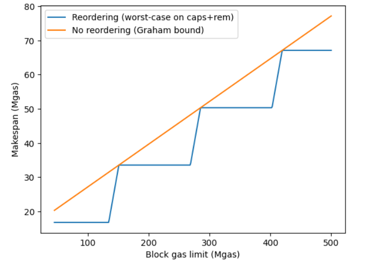
Worst-case C of OLS (orange) vs. Greedy+Reordering (blue) over increasing block gas limits using 8 threads:
Worst-case scheduling comparison for 60M block gas limit and 4 threads:
