Notes on the LVR of FM-AMM

[kosunghun317]

0. TL;DR

We introduced and detailed the additional features of FM-AMM, as presented in [CF23]. We modeled the game between CEX-DEX arbitrageurs for arbitrage profit on FM-AMM and then solved it by finding the pure strategy Nash equilibrium. Lastly, we calculated the asymptotic LVR of FM-AMM in theoretical settings and compared its performance against the Uniswap V2-style fixed-rate fee CPMM through numerical simulations. Our observations indicated that the performance is heavily influenced by price volatility, transaction costs, and the size of the liquidity pool, with FM-AMM showing a reduced loss to arbitrageurs under specific conditions.

1. Introduction

Since LVR was introduced in [MMRZ22] and [MMR23], it has quickly become the standard for measuring the performance of AMMs. Numerous attempts have been made to reduce LVR through dynamic fee policies, and this research continues actively. However, batch trade execution has not received much attention, except in [CF23] and [GGMR22]. In [CF23], the authors proposed a function-maximizing automated market maker (FM-AMM), asserting it effectively eliminates LVR, and provided numerical simulations comparing its performance with various Uniswap V3 pools. They later claimed that CoW-AMM (their implementation of FM-AMM) performed well in live settings too, which led to debate on Twitter regarding the legitimacy of their measurement methods. Although the debate focused more on whether markout is a useful metric for measuring performance, the existence of retail order flow and fluctuating transaction costs are also obstacles to precisely comparing their performance. In this article, we analyze the performance of FM-AMM and compare it to CPMM under fixed transaction costs and in the absence of retail order flow conditions like those in [N22] and [E24].

In detail, we slightly modified their design and found a Nash equilibrium in a game where arbitrageurs strategically submit orders to the (slightly modified) FM-AMM to maximize their returns. The game is similar to the liquidity provision game introduced in [MC24], which is a special form of the generalized Tullock contest. The resulting equilibrium has many favorable properties: the solution always uniquely exists, and it is symmetric. Moreover, LVR decays inversely proportionally to the number of participants. This model assumes that the number of arbitrageurs, N, is pre-determined and transaction cost, c, is zero. We proceed to a model where the number of participants is determined endogenously according to c. In this setting, FM-AMM is not always superior; the result now depends on jump size, frequency, and cost. We provide numerical simulation results and suggest that FM-AMM fits well with rollup-based solutions.

2. FM-AMM

In this section we fill the omitted details of FM-AMM introduced in [CF23] to handle the more general case. The underlying AMM curve introduced in [CF23] is:

y_\text{out} = \frac{x_\text{in}}{X + 2x_\text{in}}Y,

where x_\text{in} is the amount of token X the trader is willing to sell, and y_\text{in} is the amount of token Y that she will receive. However, this is the simplest case where only a single side of order is submitted in batch. Authors of original paper handled the case such that both side of orders exist in the same batch by assuming users only specify the amount of token X to buy or sell. Unfortunately, this is hard to implement in fully on-chain manner since whether the trader has enough capital to buy specified amount of token X is not guaranteed before the batch is settled (Selling is not problematic; we can pull the token from trader and keep it by settlement). We generalize the formula to handle broader range of cases. Let X, Y be reserves of pool, T be total supply of LP tokens before batch settlement, x_\text{in}, y_\text{in} be aggregate amount of each token that traders are willing to sell, and x_\text{mint}, y_\text{mint} be aggregate amount of each token provided from LPs. The fundamental equation we will start with is:

\begin{align}\begin{bmatrix}x_{\text{mint}} \\y_{\text{mint}}\end{bmatrix}&=x_{\text{mint}} \begin{bmatrix}1 \\p\end{bmatrix}+\begin{bmatrix}0 \\2\alpha\end{bmatrix}\\\begin{bmatrix}x_{\text{in}} \\y_{\text{in}}\end{bmatrix}&=x_{\text{in}} \begin{bmatrix}1 \\p\end{bmatrix}+\begin{bmatrix}0 \\\beta\end{bmatrix}\\\begin{bmatrix}x_1 \\y_1\end{bmatrix}&=\begin{bmatrix}x_0 \cdot \frac{y_0 + \alpha + \beta}{y_0 + 2(\alpha + \beta)} \\y_0 + \alpha + \beta\end{bmatrix}\end{align}

Here, the p is the clearing price, and \alpha, \beta are the net swap amount for swapping and minting, respectively. In short, among the submitted orders, we swap only part of them, \alpha and \beta, then exchange the rest via p2p without changing the spot price. The fact that

\begin{bmatrix}x_{\text{mint}} \\y_{\text{mint}} - 2\alpha\end{bmatrix}, \begin{bmatrix}x_{\text{in}} \\y_{\text{in}} - \beta\end{bmatrix}, \begin{bmatrix}x_1 \\y_1\end{bmatrix}

are all parallel gives us following matrix equation:

\begin{equation}\begin{bmatrix}2x_0 + 2x_{\text{mint}} & 2x_{\text{mint}} \\2x_{\text{in}} & 2x_{\text{in}} + x_0\end{bmatrix}\begin{bmatrix}\alpha \\\beta\end{bmatrix}=\begin{bmatrix}x_0 y_{\text{mint}} - x_{\text{mint}} y_0 \\x_0 y_{\text{in}} - x_{\text{in}} y_0\end{bmatrix}\end{equation}

Note that the determinant of matrix in LHS is always strictly positive so above equation is not singular. \alpha, \beta are:

\begin{align} (\alpha, \beta) = \left( \frac{\frac{x_{0} y_{mint}}{2} + x_{in} y_{mint} - \frac{x_{mint} y_{0}}{2} - x_{mint} y_{in}}{x_{0} + 2 x_{in} + x_{mint}}, \ \frac{x_{0} y_{in} - x_{in} y_{0} - x_{in} y_{mint} + x_{mint} y_{in}}{x_{0} + 2 x_{in} + x_{mint}}\right) \end{align}

The clearing price, p_c, is:

\begin{align} p_c = \frac{y_{0} + 2 y_{in} + y_{mint}}{x_{0} + 2 x_{in} + x_{mint}} \end{align}

x_\text{out}, y_\text{out} are:

\begin{align} (x_\text{out}, y_\text{out}) &= \left( \frac{y_{in} \left(x_{0} + 2 x_{in} + x_{mint}\right)}{y_{0} + 2 y_{in} + y_{mint}}, \ \frac{x_{in} \left(y_{0} + 2 y_{in} + y_{mint}\right)}{x_{0} + 2 x_{in} + x_{mint}}\right) \\ &= \left(\frac{y_\text{in}}{p_c}, p_c x_\text{in} \right) \\ \end{align}

It is straight forward to find x_2, y_2, the reserves after minting LP tokens, and t, the newly issued LP token amount, so we would skip on them here.

Above construction charges no fee. To keep price same even after charging fee, we will take 1/(1 + \gamma) portion of input and \gamma portion of output as fee. So the effective fee rate will be \frac{2 \gamma}{1+ \gamma}, which is approximately 2 \gamma. Considering arbitrageurs it may better to take fee fully on input, though.

3. Model

In this section, we describe the model upon which our analysis is based. We model a normal form game involving strategic arbitrageurs. This means that each player is unaware of the bids of others, and all bids are submitted simultaneously. Additionally, each player’s bid is never censored. Although this assumption does not perfectly reflect the current state of blockchains, ongoing cryptographic developments and improved market designs, such as inclusion lists, will help bridge the gap between theory and reality. This formulation is almost the same as that of [CM24]; the only difference is that players now “take” mispriced liquidity instead of providing it to the AMM.

3.1. Automated Market Maker

For the AMM, we will use the FM-AMM introduced in Section 2. Note that the AMM itself is not a player; we assume that the LPs of the AMM are passive investors who will not take any action in the short term.

3.2. Arbitrageurs

We assume that all players are homogeneous. They are risk-neutral and can execute trades of any size and in any direction on CEX without any slippage. Their sole goal is to maximize profit.

3.3. Strategic Game of Liquidity Taking

First, we solve the game with N players where N is given exogenously, without considering transaction costs. Then, we introduce a strictly positive transaction cost c and derive N from the equilibrium condition. We will restrict our interest to conditions with positive trading fees, which guarantees the uniqueness of the equilibrium. Players observe the pool reserves X, Y, and the external true price P. Then, they submit bids (x_i, y_i), which are the amounts of tokens to sell to the pool. The clearing price will be:

\begin{align} P_c = \frac{Y + 2\sum^N_{i=1} y_i }{X + 2\sum^N_{i=1} x_i} \tag{1} \\ \end{align}

The utility function is the arbitrage profit after charging the swap fee (and transaction cost, if applicable). The utility of player i, U_i, is:

\begin{align} U_i = -(1 + \gamma)(P x_i + y_i) + (1 - \gamma)\left(\frac{P}{P_c}y_i + P_c x_i\right) \tag{2} \end{align}

Now, we are ready to find the equilibrium.

4. Equilibrium Analysis

4.1. N is Determined Exogenously, and Transaction Cost c is Zero

We first introduce the following lemma:

\text{Lemma. The player } i\text{'s best response is submitting a bid with at least one 0 component, that is, either } (x_i, 0) \text{ or } (0, y_i).

The proof is straightforward. Assume (x_i, y_i) and (x'_i, y'_i) result in the same clearing price. Then x_i \leq x'_i if and only if y_i \leq y'_i. Combining these and subtracting the utility of one from the other yields the desired result.

Meanwhile, the first order condition and the profitability condition give us that the best response is, when P_{-i} is defined as P_{-i} = \frac{Y + 2\sum^N_{j \neq i} y_j }{X + 2\sum^N_{j \neq i} x_j}, submitting x_i or y_i such that the following holds:

\begin{align} P_c = \begin{cases} \sqrt{\frac{1 - \gamma}{1 + \gamma} P P_{-i}} & \text{if } \frac{1 - \gamma}{1 + \gamma} P \geq P_{-i} \\ \sqrt{\frac{1 + \gamma}{1 - \gamma} P P_{-i}} & \text{if } \frac{1 + \gamma}{1 - \gamma} P \leq P_{-i} \end{cases}. \tag{3} \end{align}

Otherwise, it is better not to submit any order (i.e., bid). One can think of \frac{1+\gamma}{1-\gamma}P_{-i} and \frac{1-\gamma}{1+ \gamma}P_{-i} as the threshold prices such that arbitrage becomes profitable. Note that this holds for every i, so P_{-i} = P_{-j} for every i and j, which tells us the equilibrium is symmetric and always exists.

From now on, we only consider the external price to be sufficiently higher than the pool’s spot price, Y/X. The opposite case can be solved in a similar manner. It is clear that x_\text{eq} = 0 for the case we are dealing with. Then, (3) is equivalent to:

\begin{align} \frac{Y + 2Ny_\text{eq}}{X} = \sqrt{\frac{1-\gamma}{1+\gamma}P\cdot \frac{Y + 2 (N-1) y_\text{eq}}{X}} \tag{4} \end{align}

Solving (4) yields that

\begin{align} y_\text{eq} = \frac{1}{4N^2}\left[ (N - 1) \cdot \frac{1-\gamma}{1+\gamma} \cdot PX -2NY + \sqrt{(N-1)^2 + 4N \cdot \frac{Y}{X} \cdot \frac{1+\gamma}{1-\gamma} \cdot \frac{1}{P}} \cdot \frac{1-\gamma}{1+\gamma}\cdot PX \right] \tag{5} \end{align}

From now on, we will proceed with radical approximations due to its complexity. Although we do not provide any rigorous proof for the validity of such approximations, we will see it works well in the simulations later. Let P_0 = \frac{Y}{X} and \varepsilon = \frac{1-\gamma}{1+\gamma} \cdot \frac{P}{P_0} - 1, that is, the price difference between the threshold price and the external price. Approximating y_\text{eq} with \varepsilon through a Taylor series gives us a simpler form:

\begin{align} y_\text{eq} &= \frac{Y}{4N^2}\left[ (N-1) \cdot (1+ \varepsilon) - 2N +(1+\varepsilon)\sqrt{(N-1)^2 +\frac{4N}{1+\varepsilon}}\right] \tag{6} \\ &\approx \frac{Y}{2(N+1)} \varepsilon + o(\varepsilon^2) \tag{7} \end{align}

Using (7), one can compute the profit of individual arbitrageurs and the total loss of the AMM against arbitrageurs:

\begin{align} ARB &\approx L\sqrt{P_0}\cdot\left(\frac{1+\gamma}{2(N+1)^2}\right)\cdot\varepsilon^2 \tag{8} \\ LVR &\approx (1+\gamma)\cdot L\sqrt{P_0}\cdot\left(\frac{N}{2(N+1)^2}\right)\cdot\varepsilon^2 \tag{9} \end{align}

Thus, assuming the transaction cost is 0, for any N, every N arbitrageur will submit identical bids and they will share the profit equally, while each individual arbitrageur’s profit will decay by O(N^{-2}). Moreover, as N goes to infinity the clearing price P_c converges to threshold price, and therefore the stationary distribution of price discrepancy will be as same as that of fixed fee rate CPMM in [MMR23].

4.2. Transaction Cost is Not Free, and the Number of Arbitrageurs is Determined Endogenously

Now we extend the model in 4.1 to a more realistic one by adopting a nonzero transaction cost c. The utility function remains the same as in (2), except we have an additional term -c. Since this term disappears when we take the derivative, the best response remains the same as long as it is profitable. Thus, the solution is not much different from (7), except N is replaced with N^{*}, where N^{*} is the largest integer that satisfies L\sqrt{P_0}\cdot\left(\frac{1+\gamma}{2(N^{*}+1)^2}\right)\cdot\varepsilon^2 \geq c. Then, the LVR will be:

\begin{align} LVR &\approx (1+\gamma) \cdot L \sqrt{P_0} \cdot\varepsilon^2 \cdot \frac{N^{*}}{2(N^{*}+1)^2} \tag{10} \\ &\approx cN^{*} \tag{11} \\ &\approx c \left \lfloor \varepsilon\sqrt{\frac{1+\gamma}{2c} \cdot L \sqrt{P_0}}- 1 \right\rfloor \tag{12} \\ &\leq \varepsilon\sqrt{(1+\gamma)2c \cdot L \sqrt{P_0}} \tag{13} \end{align}

4.3. Comparison with CPMM

The derivation of the LVR for CPMM has already been studied extensively, so we will simply present the result:

\begin{align} LVR_\text{CPMM} \approx \frac{1}{1-\gamma} \cdot L \sqrt{P_0} \cdot \frac{\varepsilon^2}{4}, \tag{14} \end{align}

where \gamma is the fee rate taken from the input and \varepsilon is again the price difference between the external price and the threshold price, in this case, \frac{P_0}{1-\gamma}. In short, the LVR of CPMM grows faster than that of FM-AMM as \varepsilon (the price difference) and L\sqrt{P_0} (the initial pool size) grow. From this, we can predict that the performance of FM-AMM will be better in larger pools compared to CPMM.

FM-AMM performance is affected by the transaction cost c, while CPMM is not affected as long as the arbitrageur’s profit is greater than c. This implies that FM-AMM suits well with rollup settings that have longer block times (resulting in higher volatility between blocks) and low transaction costs.

5. Simulations

Due to the nonzero transaction cost, finding an analytic solution for instantaneous LVR or the stationary distribution of price discrepancy is no longer straightforward. Therefore, we proceed with numerical simulations. You can check the code used here. This code is largely copy-pasted with minor tweaks from this source. Swap fees are fixed at 0.3% across all simulations (i.e., \gamma_\text{FMAMM} = 0.0015, \gamma_\text{CPMM} = 0.003).

5.1. Distribution of LVR

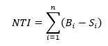
In this section, we observe the distribution of LVR under several cases without iterating over many parameters. Note that the variance is always greater in FM-AMM; this is because the price is not corrected perfectly under the nonzero transaction cost condition.

The conditions of the first case are L1 (12-second block time), $10 transaction cost, with 5% daily volatility and $100M pool size.

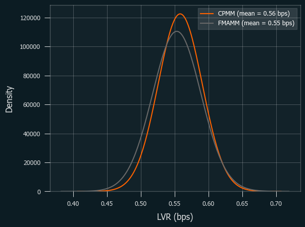
The second is L1, $10 transaction cost, with 10% volatility and $100M pool size.

As predicted, FM-AMM outperforms CPMM as volatility increases.

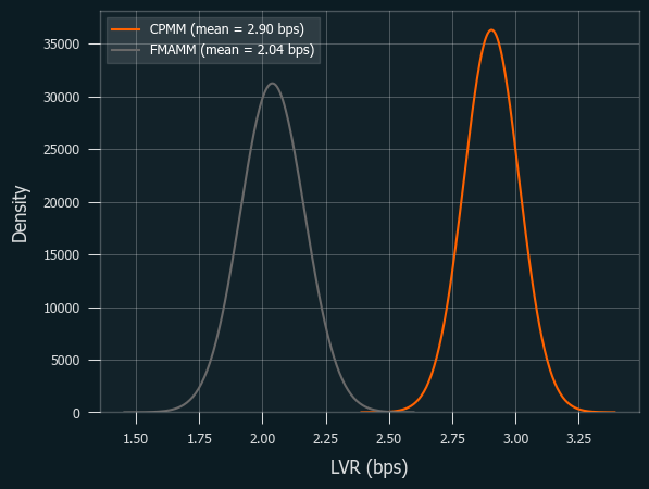
Next one is L1 with congestion; transaction cost went up to $30.

This fits to our prediction well, too. As tx cost increases FM-AMM loses more than CPMM.

The last result is L1 with congestion, but with smaller liquidity ($10M).

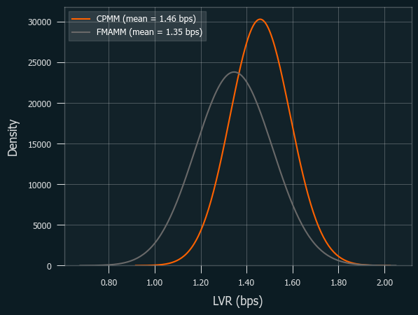
This result is a bit contradictory to our initial guess: usually, smaller liquidity conditions are more favorable to CPMM, as LVR per pool value of FM-AMM increases as the pool value gets smaller. To clarify this, we will run simulations over various parameters and compare the performances.

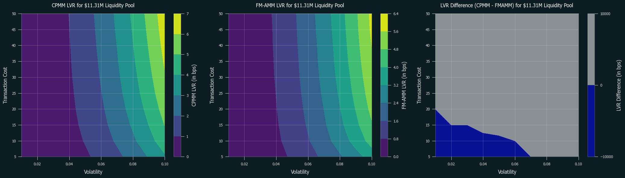
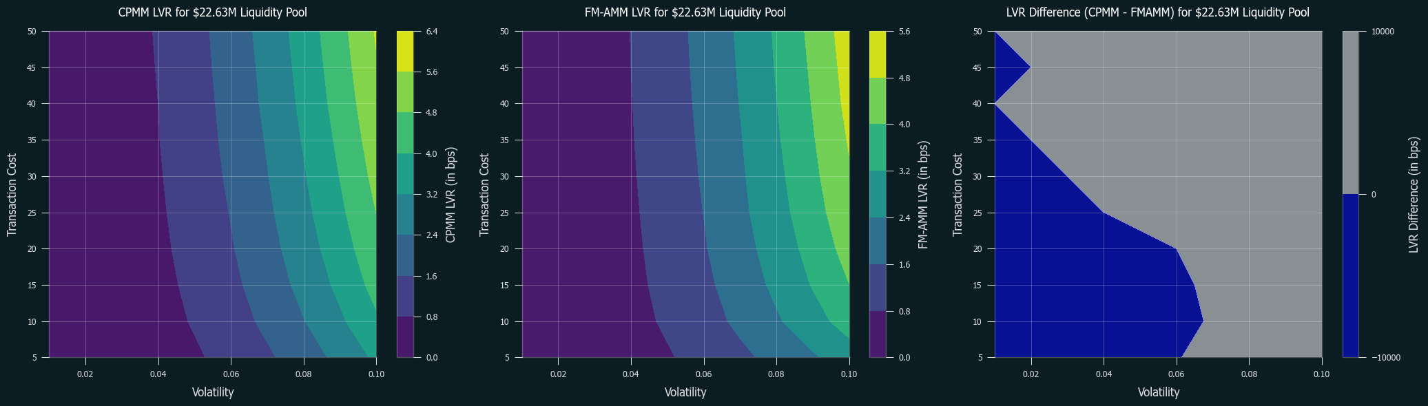
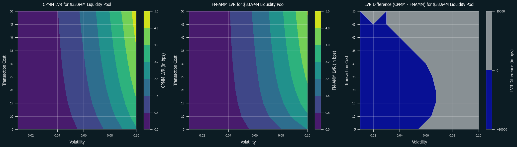
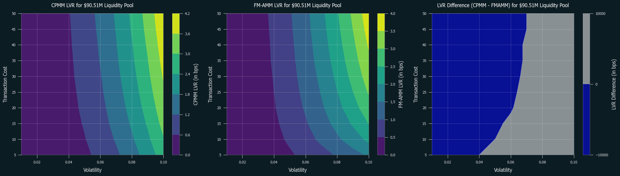
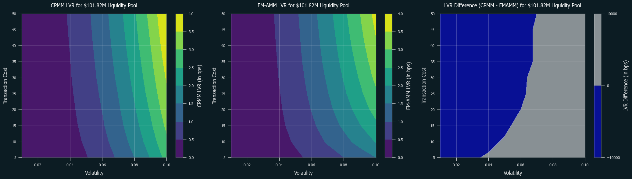
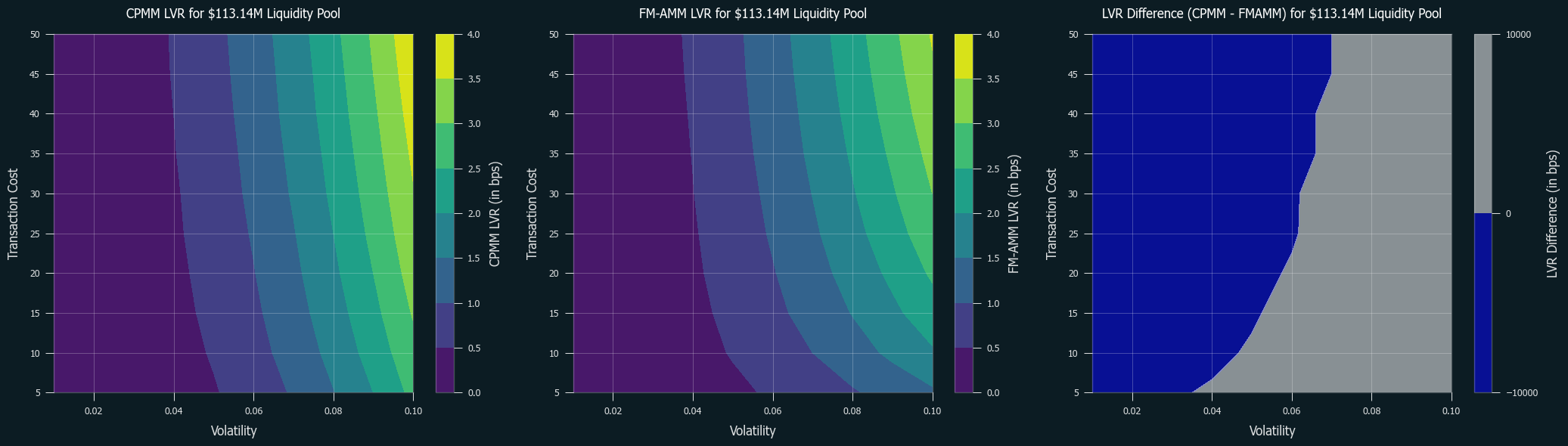
5.2. Performance Comparisons

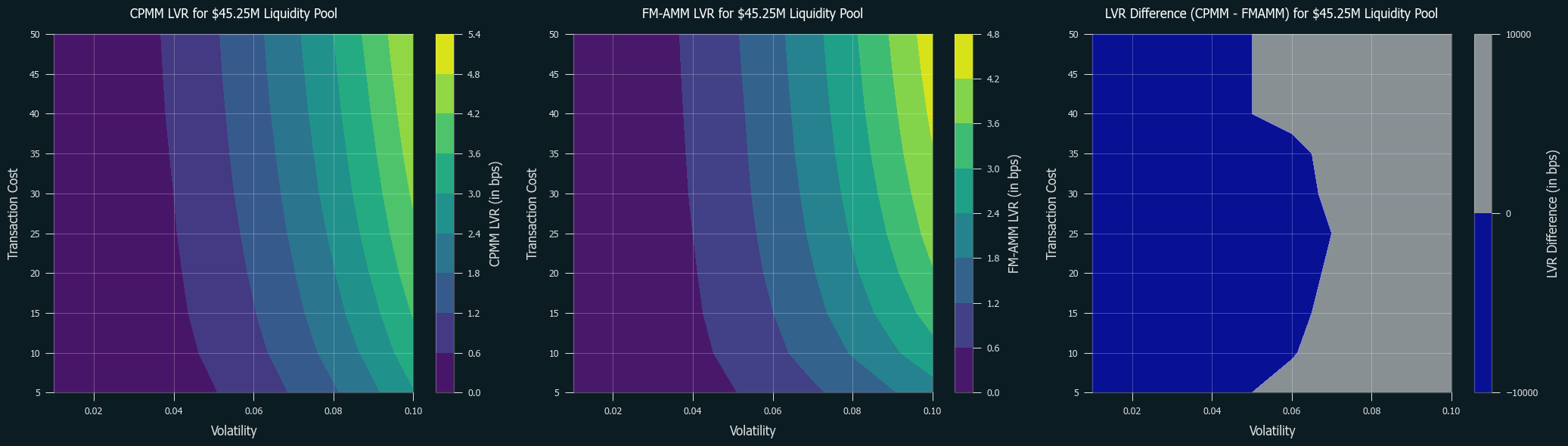
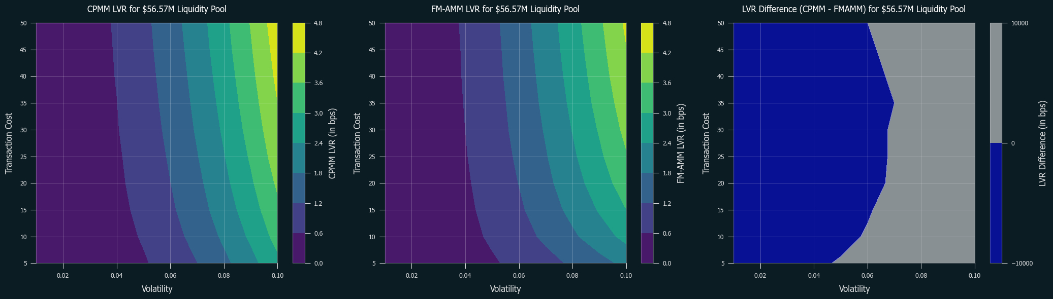
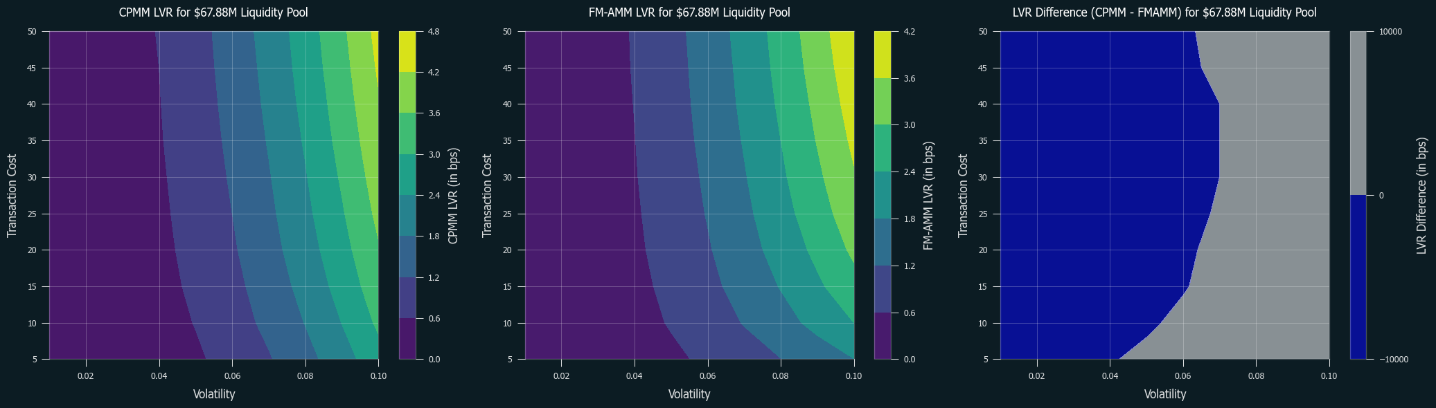
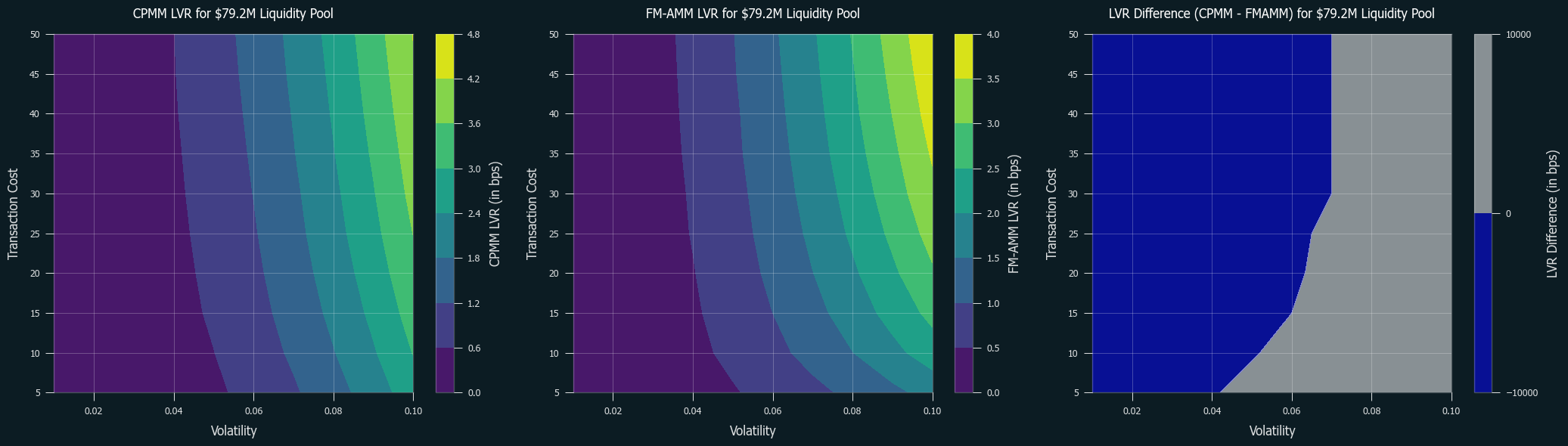
Below are the numerical simulations of LVR for CPMM and FM-AMM under various parameters. Swap fees are set at 0.3% for both of them. Blue regions indicate where CPMM performs better, while grey regions indicate where FM-AMM performs better. Note that the results in the low volatility and high-cost regions are not as reliable due to the very few trades occurring in these conditions.

First is the cases for L1:

Following are the special cases for based rollup (tx cost = $0.05, block time = 12 sec) and typical L2s (tx cost = 0.01, block time = 2 sec), respectively:

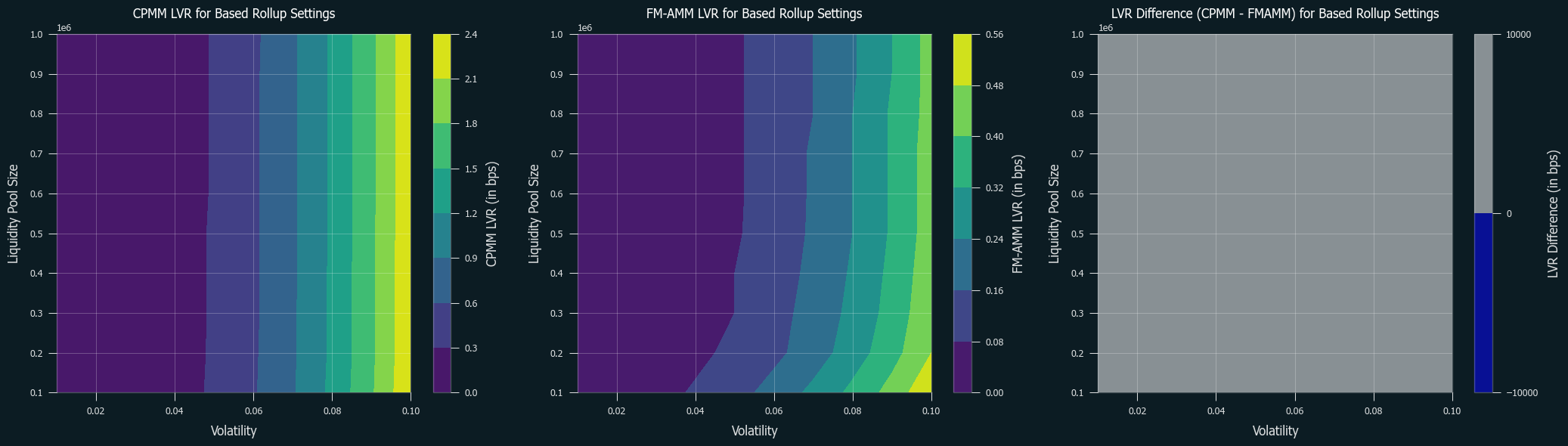
5.3. Discussion

It is clear that FM-AMM performs better under certain conditions, including L2s and L1 with low transaction costs, and this partially explains why the results in [CF23] was rather mixed and defer by each pair. Due to its nature of forcing competition over price between arbitrageurs, it performs well even in high volatility conditions. Notably, this is achieved without raising the swap fee, which typically results in losing retail order flow. Thus, FM-AMM can lose less to arbitrageurs while not sacrificing retail order flow.

6. Conclusion

As the authors of [CF23] claimed, FM-AMM indeed achieves superior performance under certain conditions, even without raising swap fees. It suits L2s particularly well. However, our analysis is based on several non-realistic assumptions, especially the (short-term) censorship resistance assumption and simultaneous bid submission. Future research will focus on more relaxed conditions to provide a more comprehensive evaluation.

7. References

[MMRZ22] J. Milionis, C. C. Moallemi, T. Roughgarden, and A. L. Zhang. Automated Market Making and Loss-Versus-Rebalancing, arXiv preprint arXiv:2208.06046, 2022.
[MMR23] J. Milionis, C. C. Moallemi, and T. Roughgarden. Automated Market Making and Arbitrage Profits in the Presence of Fees, arXiv preprint arXiv:2305.14604, 2023.
[GGMR22] G. Ramseyer, M. Goyal, A. Goel, and D. Mazières. Augmenting Batch Exchanges with Constant Function Market Makers, arXiv preprint arXiv:2210.04929, 2022.
[CF23] A. Canidio and A. Fritsch. Arbitrageurs’ profits, LVR, and sandwich attacks: batch trading as an AMM design response, arXiv preprint arXiv:2307.02074, 2023.
[CM24] D. Crapis and J. Ma. The Cost of Permissionless Liquidity Provision in Automated Market Makers, arXiv preprint arXiv:2402.18256, 2024.
[N22] A. Nezlobin. Ethereum Block Times, MEV, and LP returns, Medium article Ethereum Block Times, MEV, and LP returns, 2022
[E24] A. Elsts. CEX/DEX arbitrage, transaction fees, block times, and LP profits, Ethresearch Forum article CEX/DEX arbitrage, transaction fees, block times, and LP profits, 2024

[acanidio-econ]

Thanks for the thoughtful analysis of our work! However, I’m unclear how you calculated LVR for the CPAMM and why c does not appear in (14). You correctly say in the text that CPMM is unaffected as long as the arbitrageur’s profit exceeds c. But that implies that c should appear in the formula for LVR for the CPMM: quite trivially, if c is extraordinarily large, then arbitrageurs never trade, and LVR is zero.

A simple sanity check would be to consider the case N=1. Then, the only difference between the FM-AMM and the CPAMM is the extra “2” at the denominator of the pricing function, and comparing the level of LVR between the two AMMs should be easy. Then increasing N should decrease the LVR suffered by the FM-AMM, while leaving unaffected that of the CPAMM.

Finally, whether each arbitrageur pays c or the entire batch pays c (independently of the number of traders) is an important implementation detail. If you want to study the implementation of the FM-AMM done by CoW Swap (which we call CoW AMM), then the better assumption is that the entire batch pays c: it becomes cheaper for each arbitrageur to trade as the number of traders on the batch increases.

[kosunghun317]

Thanks for the reply. I will add more explanations below. Note that I’m using ARB for arbitrageur’s profit, that is, taking transaction cost too, while LVR, LP’s loss, does not count on it. So under my notation, LVR = ARB + c for CPMM, and LVR = ARB + Nc for FM-AMM.

@acanidio-econ

I’m unclear how you calculated LVR for the CPAMM and why c does not appear in (14).

Let external price P is greater than spot price P_0, and reserves are (X,Y) = (\frac{L}{\sqrt{P_0}}, L\sqrt{P_0}). Then arbitrageur’s profit for reporting price P_\text{rep} is:

ARB_\text{CPMM} =-\frac{1}{1-\gamma} \left( L\sqrt{P_\text{rep}} - L\sqrt{P_0} \right) - P\left( \frac{L}{\sqrt{P_\text{rep}}}-\frac{L}{\sqrt{P_0}} \right) - c.

Now the best response is reporting P_\text{rep} = (1-\gamma)P, and the profit becomes:

\begin{align} ARB_\text{CPMM} &= \frac{L\sqrt{P_0}}{1-\gamma} \left( \sqrt{ \frac{(1-\gamma)P}{P_0} } - 1 \right)^2 - c \\ &\approx \frac{L\sqrt{P_0}}{1-\gamma} \cdot \frac{\varepsilon^2}{4} - c, \end{align}

where 1 + \varepsilon := \frac{P}{\frac{P_0}{1-\gamma}}. Thus as I wrote as long as ARB_\text{CPMM} is positive LVR_\text{CPMM} \approx \frac{L\sqrt{P_0}}{1-\gamma} \cdot \frac{\varepsilon^2}{4}. Yes, as you said to be precise we should treat each profitable and non-profitable case then handle them separately. I omitted them to see the asymptotic behaviour as price gap increases, to see what happens, for instance, in extremely volatile market.

@acanidio-econ

Then, the only difference between the FM-AMM and the CPAMM is the extra “2” at the denominator of the pricing function, and comparing the level of LVR between the two AMMs should be easy.

I understand what you pointed and as you said it is rather easy to compare those in single block setting. By the complexity I meant the model in multiblock setting (i.e., this game is repeated every block while external price follows GBM) and to find an averaged rate of LVR (= \lim_{T \rightarrow \infty} \frac{\int^T_0 LVR_t dt}{T}) since price after equilibrium is not set as threshold price in the presense of transaction cost. I’m working on it but math looks quite complicated, and that’s why I replaced it with numerical simulations. Since I only know basic things about probability this maybe not a hard task to others.

@acanidio-econ

Finally, whether each arbitrageur pays c or the entire batch pays c (independently of the number of traders) is an important implementation detail.

Yes I’m aware of that (I’m using cowswap everyday and even LP’d on GNO/COW pair too!) and that would indeed improve the performance. However that would need an operator who aggregates bids off-chain and settle the batch. I wanted to consider something that does not need off-chain operator and works even without such operator so that it can be easily forked and used in many chains, not the exact implementation of CoW AMM. Of course but then my setting will still rely on some centralized setting since satisfying sealed bid condition is currently impossible without relying on TEE or FHE. So the setting I choosed to work with was picked based on my personal preference, which is not reflecting the reality nor ease of implementing in realistic assumptions.

[acanidio-econ]

@"kosunghun317

So under my notation, LVR = ARB + c for CPMM, and LVR = ARB + Nc for FM-AMM.

Probably just a typo, but I think it should be LVR = ARB + N^* c for FM-AMM. It is important to keep in mind that because N^* can take any value below N (including 1), in both the FM-AMM and CPAMM. an arbitrageur wants to trade if the profits from doing it are greater than c.

@"kosunghun317

Yes, as you said to be precise we should treat each profitable and non-profitable case then handle them separately. I omitted them to see the asymptotic behaviour as price gap increases, to see what happens, for instance, in extremely volatile market.

The problem is not so much about looking at the asymptotic behavior. It is that you do so only for the CPAMM and not for the FM-AMM, which creates an asymmetry between how you compute LVR for the two cases: in one case, you say that the cost c is small relative to the volatility and can be ignored, in the other case instead you explicitly account for it. It then becomes hard to interpret the simulations for the case high c / low volatility.

@"kosunghun317

I’m working on it but math looks quite complicated, and that’s why I replaced it with numerical simulations. Since I only know basic things about probability this maybe not a hard task to others.

I wasn’t suggesting a full analytical solution. Rather, you may try to simulate the LVR of a CPAMM by taking the code you already developed for the FM-AMM, setting N=1, and adjusting the pricing function. Doing so, you should get an “exact” calculation where c is properly taken into account, both for the CF-AMM and for the CPAMM. Then the comparison between the two is more meaningful.

@"kosunghun317

So the setting I choosed to work with was picked based on my personal preference, which is not reflecting the reality nor ease of implementing in realistic assumptions.

Sure, but youy started your post by discussing CoW AMM and the debate around its performance, If you want to contribute to that debate, then the correct assumption is that c is paid by the entire batch. Of course, it is also interesting to study a hypothetical future implementation of FM-AMM that is fully decentralized and in which gas in paid by each trader separately.

[kosunghun317]

@acanidio-econ

It is that you do so only for the CPAMM and not for the FM-AMM, which creates an asymmetry between how you compute LVR for the two cases

Yes I made a mistake while explanation and it may sound like I applied nonzero cost c only for FM-AMM. The correct LVR of CPMM would be:

LVR_\text{CPMM} = \begin{cases} \frac{L\sqrt{P_0}}{1-\gamma} \cdot \frac{\varepsilon^2}{4}, & \text{if } \frac{L\sqrt{P_0}}{1-\gamma} \cdot \frac{\varepsilon^2}{4} \geq c \\ 0, & \text{else} \\ \end{cases}

And similarly we can find the LVR of FM-AMM in more precise manner. Although I was sloppy on post but I correctly took account of cost for both of case and I’m pretty sure that I don’t have run the simulations again with fixing N=1 for sanity check. You can check code block [5] and [6] of my notebook.

@acanidio-econ

Sure, but youy started your post by discussing CoW AMM and the debate around its performance, If you want to contribute to that debate, then the correct assumption is that ccc is paid by the entire batch.

This sounds correct. I will add the result with that condition later.

[laurentyzhang]

There is a another approach. The idea is to balance buy and sell orders in batch to keep slippage within a predefined tolerance level set by the platform. The solution has three major steps:

• First, the platform gathers incoming transactions over a predefined period and selects them based on the “neutral” principle, ensuring that the sum of buy and sell orders is proportionally balanced relative to the pool’s liquidity.

• Second, the platform matches these orders to maintain balance.

• Finally, the unmatched transactions will be held for the next batch, processed with a higher slippage tolerance, or refunded to the user, depending on their preference.

Proportional Impact Calculation: The goal is to ensure that the impact of a batch of transactions on the AMM pool is proportional to the liquidity of the pool. This is achieved by ensuring that the Net Transaction Impact (NTI) relative to the pool’s liquidity (L) is below a certain threshold.

Net Transaction Impact (NTI): Let B_i and S_i represent the buy and sell orders in a batch, respectively. The Net Transaction Impact (NTI) is defined as:

The condition for the “neutral” batching process is that the ratio of NTI to the pool’s liquidity L should be less than a threshold value k:

where k is a constant that represents the maximum allowable impact as a proportion of the pool’s liquidity. This ensures that for larger pools, a larger NTI is acceptable, whereas for smaller pools, the NTI must be smaller to avoid significant price shifts.

Execution and Settlement: Once a “neutral” batch is formed within the proportional impact threshold, the transactions will be executed simultaneously, with the AMM adjusting the pool’s reserves accordingly. This dynamic adjustment helps maintain price stability while accommodating varying liquidity levels.