A problem that often appears in optimizing ZK-SNARK implementations, Ethereum clients, and other cryptographic implementations is as follows. You have a large number of objects (usually elliptic curve points) P_1 ... P_n, and for each object you have a correspondting factor f_1 ... f_n. You want to compute P_1 * f_1 + P_2 * f_2 + ... + P_n * f_n, and do so quickly.
Many people (ab-)use the term “Pippenger algorithm” to refer to a whole family of fast-linear-combination algorithms; this post takes you through the basic idea of how they work and includes a code link to a limited but simple such algorithm.
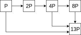
Naively, assuming a 256-bit group order, computing a linear combination of N points takes \approx 384 * n point additions using the square and multiply: for each value P_i, keep doubling it to generate 2P_i, 4P_i, 8P_i etc etc until you get to 2^{256}P_i, and then add together the subset of those values that correspond to 1 bits in the factor (on average half of the bits will be 1, hence add another 128 point additions to get 384). For example, if your factor is 13, then 13 in binary is 1101, so you would add P_i + 4P_i + 8P_i.
But if we have more than one point, can we do better? It turns out that yes we can. First of all, we’ll start with an algorithm that gets us a modest 3x improvement. This algorithm works by converting a linear combination problem into a “multi-subset” problem.
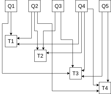
The multi-subset problem is described as follows: given a set of points Q_1 ... Q_n, compute the sum of the values in each subset S_1 ... S_k where S_i \subset \{Q_1 .... Q_n\}. For example, given Q_1 ... Q_5, we might want to compute the sums of each of the subsets (\{Q_1, Q_2, Q_4\}, \{Q_2, Q_3, Q_4\}, \{Q_1, Q_3, Q_4, Q_5\}, \{Q_2, Q_4, Q_5\}). In those case we would want four sums (which we’ll denote T_1 ... T_4), one for the values in each subset, eg. T_1 = Q_1 + Q_2 + Q_4.
Now here is how we convert a linear combination problem into a multi-subset problem. Take d subsets, where d is the number of bits in the highest factor in binary (often d = 256), where the i’th subset is the subset of points whose corresponding factors have an i’th bit of 1. For example, for the factors \{5, 11, 6, 15, 12\}, the first subset is the subset corresponding to the odd factors, so \{Q_1, Q_2, Q_4\}, the second subset is the subset whose 2’s bit is 1 (ie. which are 2 or 3 mod 4), so \{Q_2, Q_3, Q_4\}, and so on (yes, I chose the factors deliberately to match the example above).
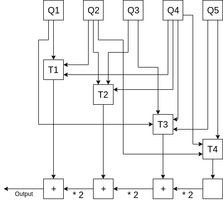
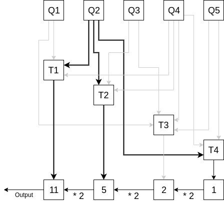
Now, here is how we compute our desired linear combination 5Q_1 + 11Q_2 + 6Q_3 + 15Q_4 + 12Q_5. Let T_i = sum(S_i) where S_i is the i’th subset (so eg. T_1 = Q_1 + Q_2 + Q_4). Notice that the desired linear combination exactly equals T_1 + 2T_2 + 4T_3 + 8T_4. To see why this is the case, consider the number of times any given factor appears, eg. Q_2 (with a corresponding factor f_2 = 11). 11 in binary is 1011, so its 1st, 2nd and 4th bits are turned on. Hence, it has a presence in T_1, T_2 and T_4, and so it is present 8 + 2 + 1 = 11 times in T_1 + 2T_2 + 4T_3 + 8T_4. We can repeat the same argument for every Q_i, and so every Q_i appears in the final sum the correct number of times.
We compute T_1 + 2T_2 + 4T_3 + 8T_4 efficiently with a double-and-add chain:
We can verify that Q_2 shows up 11 times graphically by only paying attention to what multiple of Q_2 is represented at each step:
For 256-bit factors and n points, this procedure has a cost of 256 * 2 = 512 operations for the bottom row, plus 128 operations, on average, to compute each subset, so we get a cost of 512 + 128n operations; as n gets large this approaches being three times as efficient as the naive approach of computing every product and adding them at the end separately.
Now, let us get to more efficient ways of solving the multi-subset problem. In the example above, naively computing (\{Q_1, Q_2, Q_4\}, \{Q_2, Q_3, Q_4\}, \{Q_1, Q_3, Q_4, Q_5\}, \{Q_2, Q_4, Q_5\}) would cost 2 + 2 + 3 + 2 = 9 operations: |S_i|-1 operations for each subset S_i. But notice that there are partial computations that we can merge. If we first compute R_1 = Q_2 + Q_4, then we reduce the remaining calculation to (\{Q_1, R_1\}, \{Q_3, R_1\}, \{Q_1, Q_3, Q_4, Q_5\}, \{R_1, Q_5\}), which cuts us down to 1 + (1 + 1 + 3 + 1) = 7 operations. In general, the more subsets you have, the more mergings you can do. For example, if you have many subsets each having about half of some list of elements (which is our situation), then any randomly selected pair of elements will on average appear in about a quarter of the subsets.
The various more efficient ways of solving the multi-subset problem, which in turn lead to fast linear combination algorithms using the method described above, basically have to do with coming up with different heuristics for figuring out which subsets to compute first to achieve the largest reduction in total computation.
In research/fast_linear_combinations/multicombs.py at 420a19e4449a2a85cb81a6731d6cf4534c3a366b · ethereum/research · GitHub I made a fairly simple implementation: search through all pairs to find the pairs that appear in the most subsets, add new elements for them, and repeat until there are no more pairs.
This algorithm does have the problem that it requires O(n^2 * log(n)) “bit-twiddling” work, which eventually overcomes the benefit of the O(N / log(N)) operation count for making a N-element linear combination. However, for inputs up to size ~100 this extra work is small, and at those levels you get a further ~2.5x improvement compared to the “simple” multi-subset approach (ie. ~7.5x improvement relative to multiplying each point separately), and for larger inputs you can just split them up. There are more advanced algorithms (eg. see here), but this is beyond the scope of this post; this very simple algorithm seems able to get you to within half of the theoretical optimum in most practical cases.


