In econ it’s well known that “ambiguous devices” have all kinds of useful and interesting mechanism design properties (e.g. see this 2024 Econometrica). It turns out that a blockchain + a pathological RNG called Machine II can create a very general purpose “ambiguous device”. You can see a demo running in a TEE here.
Here’s the idea for AMMs. Suppose we treat LPing as a classic Exclusion Game in which the LP wants to make profit but traders can “exclude” you from the profitability region (LVR let’s say). The game models the dilemma for the LP as basically:
Charge high fees to get some arbitrage protection, but at the risk of scaring off retail.
Charge low fees to attract retail but get arbed.
It turns out that in such a game, using an ambiguous device (“veiling your fees”) can really improve the situation for the LP. The math can be a little tedious and unfamiliar, so I think it’s useful to show pictures of what veiled fees do to the game.
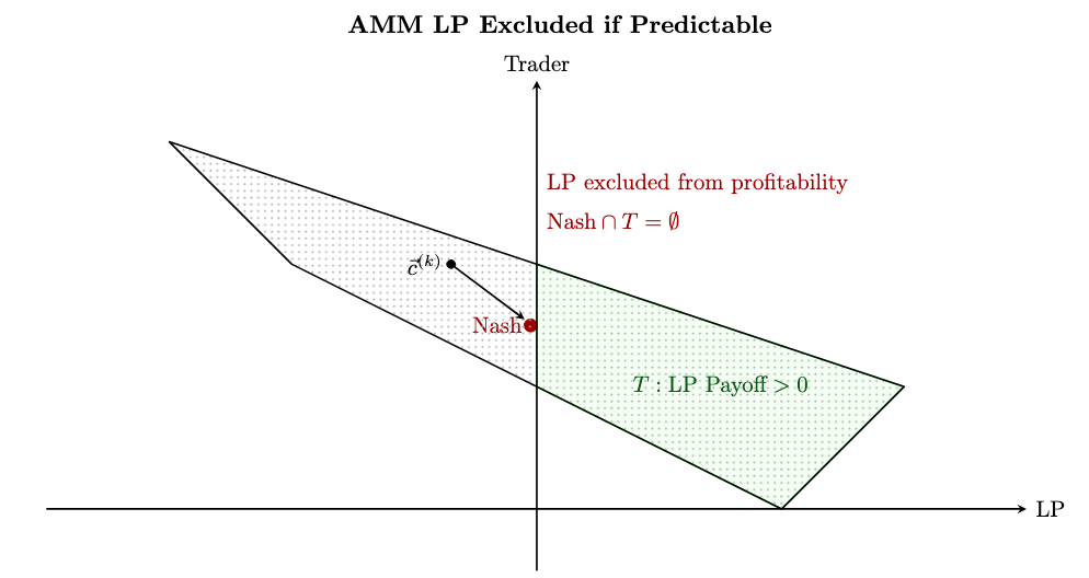
Below is the “problem picture”, showing that the LP has no viable strategy to be profitable. The unique Nash Equilibrium pays \le 0 and so they are excluded from the green region (T).
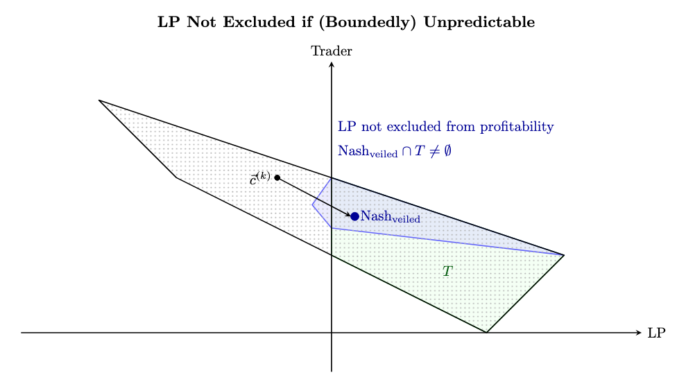
When you introduce veiled fees the LP’s payoffs are not fixed but now lie in the full blue region. Clearly LP is no longer excluded from profitable region T (in fact they can even reach the highest possible payoff way off to the right.) Further, the blue region is clearly truncated on the left, so the LP risks very little for this.
To establish actual payoff numbers, one needs to make an assumption about how exactly the LP treats their payoff uncertainty. Obviously the LP would have to be pretty averse to uncertainty to not see the blue region as an improvement over the Nash in the earlier figure.
If we assume neutrality for the LP, such that their best and worst payoffs are evaluated at the halfway point, the LP improves their payoffs from 0 (under the Mixed Nash) all the way to 1.4 (under the Veiled Nash).
You can read more in the draft paper here. I will say I’ve run this approach by a decent proportion of the high end crypto brain trust at this point and thus far no substantial objections have been raised. It’s a little shocking to some that you can pareto dominate a unique mixed strategy Nash Equilibrium (it was to me when I first saw it) but here in 2025 this is mainstream–if cutting edge–game theory.
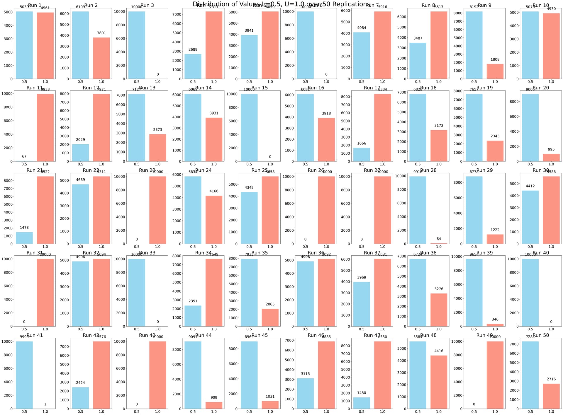
Even though each individual Machine II sequence doesn’t converge to a single average, the expected value across all Machine II sequences at any position would have some definite value expected by the trader. If the selection process of the veiled sequence is truly random and unbiased, this expected value would be 0.75 when the range of possible outputs is [0.5, 1.0]. The trader always expects a 75% chance of highfee. Thus the informed trader is able to use a mixed nash which you demonstrated does not contain profit for the LP.
The issue is the random selection of a Machine 2 sequence undoes the benefits of using an unpredictable sequence. For a visualization imagine plotting the Y outputs of an infinite number of machine II sequences that stay between 0,5 and 1. Now every location on the x axis would be equal density for every Y value meaning using a randomly selected unbiased machine 2 sequence [0.5, 1.0] is the same thing as just picking high fee with 75% odds.
Lens: I read the entire paper, I am a game theoretic mechanism designer of 8 years experience, and I have ran into this situation before where randomness at a higher level overrides the lower level.
Thanks for giving it a read. Maybe the LVR draft isn’t clear enough about how Machine II is being used (the other paper directly about Machine II is more comprehensive.) Committing to an encrypted Machine II draw to resolve the exchange is where the EV-denying magic is. Certainly revealing the RNG ahead of time would not work
The non-convergent sequence is what denies vanilla expected value approach. And in most cases if the trader just responds ‘as if’ it was a mixed strategy they will do worse. Also worth noting that there are veiled equilibria where both players do better-- for instance if the LP veils over (.450,1) then the trader gets .50 more (and the LP gets .25 less.)
NP. I initially responded from my phone half asleep. I will try to make my point clearer so we can find the misunderstanding or disagreement.
I understand it is used to resolve the exchange after committing to trade, and not revealed ahead of time.
I understand that this relies on a non-convergent sequence that would result in the trader being unable to pick a probability that is profitable even when averaging over a long time span. It could be lowFee for a year straight or highFee for 10 years straight and no timespan is long enough to find an average.
Consider the traders perspective on a single trade. The LP is choosing lowFee or highFee using a machine II sequence bounded between [0.5, 1]. The LP has secretly selected from an infinite number of Machine II sequences, choosing Sequence S. I assume the set of Machine II sequences has no built in bias towards some output. Consider the probability of the first output of this sequence being between 0.5 and 0.6. It is 20%. The same goes for 0.7 to 0.8 , 20%. There is equal probability of selecting each probability. Thus the probability the first trader faces of getting highFee is 75%, the same as if the LP just choose a random number from 0.5 to 1. If you average together the * next * output of an infinite number of machine II sequences bounded from 0.5 to 1, the average will be exactly 0.75.
I really don’t like using AI as it usually gets stuff like this wrong, but here is Claude’s attempt to explain the above more academically:
The paper assumes that using a non-convergent sequence (Machine II) bounded between [0.5, 1.0] creates an advantage over a standard mixed strategy with p* = 0.75. However, from the trader’s perspective, if the LP randomly selects from all possible Machine II sequences without bias, the expected probability of high fees on any individual trade remains 0.75.
The core issue is that randomizing over non-convergent sequences doesn’t eliminate the trader’s ability to form rational expectations about the next trade. While individual Machine II sequences don’t converge to a single average, the distribution of possible outcomes for the next trade does have a well-defined expected value (0.75).
The random selection of a Machine II sequence creates a meta-distribution with mean 0.75, functionally equivalent to the mixed Nash equilibrium from the trader’s decision-making perspective
The trader doesn’t need to know which specific sequence was selected to optimize their strategy - they only need the expected probability for the upcoming trade
If people prefer to treat that output as exactly the same as 500k coin flips they definitely can, and then it would look like the mixed strategy Nash outcome as you say. Nobody is worse off. But if people treat Machine II as what it actually is–a souped up cauchy oscillator with no expected value–then the efficiency gains highlighted above become possible.
But note that both cases above, coin flip and cauchy, will still technically stem the players’ preferences and not just their rational beliefs. More colorfully, you could say that in both cases veiling has changed an information arbitrage game into a preferential exchange game.
It does seem surprising that doing this can make both players better off! One intuition for how it works is that it’s letting players kind of ‘trade their corners’ in a more expressive way. It’s a bit of a rabbit hole, but fyi it isn’t wild heterodox stuff. To respond to your AI message above: if we ask the question more directly, Claude does get it right:
“Does a non-convergent series have a single expected value?”
A non-convergent series doesn’t have a single expected value.
When a series doesn’t converge, its partial sums don’t approach any fixed finite value. This means we can’t assign a single number as the “expected value” or “sum” of the series.
If you’d prefer to use the actual math for Machine II, it’s this: for every \epsilon>0 and sufficiently large k,
Yes, a single non-convergent series does not have a single expected value. The trader however is not faced with a single non-convergent series. They are faced with a random selection of non-convergent series making the average expected next output converge to exactly 0.75. It appears the primary point of disagreement is that I believe the non-convergence is undone by the random selection of machine II sequences and you do not. The missing step in this paper is taking an infinite number of machine II sequences and average together the output.
Claude attempts a formal proof the next output converges to 0.75 when randomly selecting among non-convergent series:
Let’s define our scenario precisely:
Let 𝒮 be a set of non-convergent series, where each series S_i ∈ 𝒮 has all terms bounded between 0.5 and 1.
Let R be a random selection process that chooses series from 𝒮 according to some probability measure μ.
Let M be the resulting meta-distribution.
Proof that M is convergent:
First, observe that while each individual series S_i ∈ 𝒮 is non-convergent, each term in every series is bounded between 0.5 and 1. This means that for any series S_i = (a_1, a_2, …), we have 0.5 ≤ a_j ≤ 1 for all j.
When we randomly select a series according to the probability measure μ, we’re effectively creating a weighted average of the behaviors of all series in 𝒮.
Let’s denote the random variable representing the nth term of a randomly selected series as X_n. The expected value E[X_n] is: E[X_n] = ∫_𝒮 S_i(n) dμ(i) where S_i(n) is the nth term of series S_i.
Since all terms are bounded between 0.5 and 1, we know: 0.5 ≤ E[X_n] ≤ 1 for all n.
Furthermore, the variance of X_n is bounded because: Var(X_n) = E[(X_n - E[X_n])²] ≤ E[(1 - 0.5)²] = 0.25
By the law of large numbers, as we increase the number of random selections, the empirical distribution of the terms converges to a well-defined probability distribution. This distribution is our meta-distribution M.
While each individual series diverges, the meta-distribution M captures the statistical properties across the ensemble of series. The key insight is that M doesn’t represent the limit of any particular series (which would diverge), but rather the distribution of terms at each position across all possible selected series.
Since both the expected value and variance of X_n are bounded for all n, the central moments of the meta-distribution M are all finite.
By the theory of statistical convergence, even though each individual series diverges, the meta-distribution M converges to a stable distribution that characterizes the statistical behavior of randomly selected terms from our set of non-convergent series.
This convergence is in the sense of distributional convergence, not pointwise or uniform convergence of the underlying series themselves.
Therefore, the meta-distribution M formed by randomly selecting from non-convergent series bounded between 0.5 and 1 is convergent in the distributional sense, even though each individual series diverges.
This demonstrates an important principle: collective statistical behavior can exhibit stability and convergence even when individual elements display divergent behavior.
Not sure where the idea came from that Veiling is about averaging sequences. It is not–the mathematical properties of the machine are cryptographically attested to so people have the correct prior(s) on the next draw from the machine. And that prior is, as you note, not a pure expected value. It happens that Machine II has a few more bells and whistles so it can resist learning over time (and thus can be used at scale) but that might be a distraction for this convo.
The really interesting properties come from what you can do with the bounds though. Will write some more about that later but wanted to make sure to get past the EV question first.
The protocol presented here involves a non-convergent series chosen at random. The selection process of the machine II sequence is what changes the convergence back to 0.75. The trader doesn’t know which sequence was selected and expects exactly 0.75 because of how the sequence is selected. Even though reality is (machine II)=? the trader always sees (uniform random selection of (machine II)) which equals 0.75.
If you want to refute my criticism it would require arguing that the random selection of a machine II sequence does not itself cause convergence. I have given multiple arguments regarding this and none of them are responded to, instead you reiterate the properties of a single non-convergent series.
“Does a non-convergent series have a single expected value?” NO
“Does randomly selecting from an infinite number of non-convergent series where outputs are bounded from negative infinity to positive infinity have a single expected value?” NO
“Does randomly selecting from an infinite number of non-convergent series where outputs are bounded between two numbers have a single expected value?” YES
I claim to get convergence out of non-convergent series it requires two things: selecting from an infinite number of non-convergent series and the outputs of these series are all bounded between two numbers and uniformly distributed between those numbers. If both are true the expected value converges to halfway between those number bounds. Your protocol does both of these things. Consider the very first output of your protocol, the trader expects exactly 0.75 and the average first output will be 0.75.
convergence out of non-convergent series it requires two things: selecting from an infinite number of non-convergent series and the outputs of these series are all bounded between two numbers and uniformly distributed between those numbers.
Neither of these conditions hold here. Let’s move on and stop bumping the thread for basic stats questions. Feel free to DM.
I lose track around when you are discussing a “veiled equilibrium” and cite Keeney and Raiffa (which I haven’t read). I think there is some unusual type of game theory happening here related to your initial comments about ambiguity.
Can you clarify – it sounds like the LP commits to this non-stationary sequence, and then the trader responds how? I would normally think that once the LP commits, at each round, the trader forms a Bayesian belief over the next price from the machine and best-responds to that belief. This might be what imkharn is thinking as well. But it sounds like somewhere here, the “veiling” magic happens and the trader behaves in a different way…
Thanks for the response. The terminology can be a little bit of a distraction, but just to be clear Veiled Equilibrium is the name for “commitment + ambiguous device”. It’s most similar to Binmore’s “muddled equilibrium”, which it draws on.
But the game theory itself is more cutting edge than fringe. For some intuition (which you personally probably do not need), mixed strategies were introduced in Game Theory as “random devices used to conceal one’s behavior”. The idea that ambiguity offers better concealment, and so may be advantageous, thus makes some sense right off the bat. And then for the domain of application, it’s well known that positive sum games have weird and sometimes unconvincing Nash Equilibria. Which is all to say that this paper and Machine II more generally is not so strange even by textbook game theory standards.
And then for your second question: the trader will form a Bayesian belief but rationally it must condition on an ambiguous Machine II draw. Thus will necessarily involve multiple priors that do not collapse to a single traditional EV. Of course, the trade will ultimately resolve at a single value, and so collapsing must take place somewhere. Here you can use ambiguity models, as I do in the main Machine II paper, or you can use supporting visual intuition about the game as I do above. Overall though, the math is telling us the behavior can be Pareto improving, with no incentive to unilaterally defect, and can thus presents a good candidate for equilibrium selection. Beyond that, more work and experimentation needs to be done. This is underway, not just by me
I have learned that the set of machine II sequences ITSELF is non-convergent, so the “selection from an infinite number of non-convergent series” is itself a non-convergent process. Even on a meta level before the convergent series is selected there is no expected mean. This means that even if you pick a new machine II for every trade, there is still no mean or EV. When you kept responding to me with the properties of Machine II, I thought you were missing my point. I was assuming that the properties of Machine II stop becoming relevant if they are selected at uniform random, but what I didn’t know was that the properties of Machine II also include the distribution of the sequences in the set that you would randomly select from… it is non-convergent even on a meta level.
Side note: While investigating this, Grok noticed a different issue that seems like it might be valid. I will share its summary:
Even if the mathematical construction successfully prevents a classical EV, 0.75 is such a strong Schelling point that traders may coordinate on it anyway. Once that happens (even though on paper it was irrational to do) , it could become self-reinforcing. If enough traders start using 0.75 as their working assumption (because it’s focal and “good enough”), then:
It becomes rational for other traders to also use 0.75, because they expect others to use it.
Once this coordination happens, deviating from it (e.g., trying to exploit the true ambiguity or acting more conservatively) can become irrational in the short-to-medium term, because the other side is already playing as if it’s 0.75.
You end up in a self-reinforcing equilibrium that is stable, even though getting there may have required players to ignore (or be unaware of) the deeper technical features of Machine II.
This equilibrium might be meta-stable — once you’re in it, it’s hard to escape, even if the original design intent was to keep agents in the ambiguity regime.