The ECFFT algorithm (without elliptic curve and isogenies!)
thanks to William Borgeaud for helping me understanding the original ECFFT algorithm
tl’dr: this post is for people that would like to understand the mechanics of the new ECCFFT algorithm without have any knowledge of isogenies and elliptic curve (of course this is not a suggestion to not learn isogenies ![]() , in case you want here you can find a thread I have done). Mind that this makes sense ONLY for learning purposes indeed from the performance point of view there is no gain to go this route.
, in case you want here you can find a thread I have done). Mind that this makes sense ONLY for learning purposes indeed from the performance point of view there is no gain to go this route.
For a background about classic FFT algorithm I suggest to read Vitalik’s post. The classic FFT algorithm leverages the 2-adic evaluation over finite fields.
What does it actualic means? Simply that we want to have a large power of two root of unity in the field F_p. More precisely if we are working over F_p we want that the order (in this case being p a prime number the order is “simply” p-1) is divisible by an high power of 2.
Recently Eli Ben-Sasson, Dan Carmon, Swastik Kopparty and David Levit published a clever FFT algorithm that generalizes the classic FFT and is based on 2 isogenies (rather than power of 2 over F_p)
The ECFFT algorithm
A quick summary of the algorithm is the following (assuming we want to do FFT over F_p):
- the first step is to find a suitable curve over F_p that has a nice order (i.e. the number of points - aka the order - is divisible by a big power of 2, let say 2^n).
- there is a precomputation phase where the 2^n points points are correlated to the isogenies. This is achieved by using a polynomial decomposition built over the isogeny’s rational polynomial (yes an isogeny is a rational polynomial) that is a bit more complicated than the classic finite field.
- Then a set of fast algorithms for working with polynomial can be implemented (with the routine called
extendbeing the base for many others routines)
William Borgeaud did a great job implementing the ECFFT algorithm both in Rust and Sage. Kudos.
The following part of the post is going to “translate” the simple example found in Vitalik’s post using the modified ECFFT algorithm adjusting William’s Sage code.
The ECFFT algorithm
The motivation for writing this post came directly from Section 3 of the original paper:
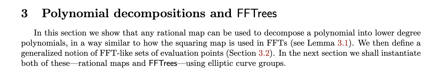
As you can read above it states that
any rational map can be used to decompose a polynomial into lower degree polynomials
The ratonal map used in the ECFFT is a bit convoluted (it is not really simple to compute P_0 and P_1 and not even needed to do for the algorithm to work), leverages the Lattés maps for isogenies and looks like:
this is translated in sage’s code as the matrix
M = Matrix(F, [[v(s0)^q,s0*v(s0)^q],[v(s1)^q, s1*v(s1)^q]])
Mind you do not need to understand this, well this is the only purpose of this post overall
The rational map in the finite field case is instead really simple. Indeed as explained in Vitalik’s post it is “enough” to split the polynomial P in even-degree coefficients (let’s call it P_0) and odd-degree coefficients (P_1) and reconstrcging the original polynomial is as simple as
this is reflected in the new matrix becoming:
M = Matrix(F, [[1,s0],[1, s1]])
Also the precomputation part is way more simple.
There indeed no need to precompute the isogenies but it would be enough to split the evaluation values (two root of unity in this case):
S = [1, 148, 336, 189]
S_prime = [85, 111,252, 226]
and the precompute is just storing the needed transformation matrix in memory (the loop is performed over square root modulo p rather than isogeny walk).
The beauty now is that the other algorithms extend and enter remain immutate.
You can find the complete code below and in this gist
# p and values taken from the example https://vitalik.ca/general/2019/05/12/fft.html
# based on the work https://solvable.group/posts/ecfft/
p =337
F = GF(p)
log_n = 3
n = 2^log_n

S = [1, 148, 336, 189]
S_prime = [85, 111,252, 226]

cosets = {}
cosets[0] = [1, 85, 148, 111, 336, 252, 189, 226]
cosets[1] = [1,148,336,189]
cosets[2] = [1,336]

def precompute(log_n, S, S_prime):
    Ss = {}
    Ss_prime = {}
    matrices = {}
    inverse_matrices = {}
    for i in range(log_n, -1, -1):
        n = 1 << i
        nn = n // 2
        matrices[n] = []
        inverse_matrices[n] = []
        R2.<X> = F[]
        for j in range(nn):
            s0, s1 = S[j], S[j + nn]
            M = Matrix(F, [[1,s0],[1, s1]])
            inverse_matrices[n].append(M.inverse())

            s0, s1 = S_prime[j], S_prime[j + nn]
            M = Matrix(F, [[1,s0],[1, s1]])
            matrices[n].append(M)

        S = [(x^2 %p) for x in S[:nn]]
        S_prime = [(x^2 % p) for x in S_prime[:nn]]

    return matrices, inverse_matrices

# Precompute the data needed to compute EXTEND_S,S'
matrices, inverse_matrices, = precompute(log_n-1, S, S_prime)

def extend(P_evals):
    n = len(P_evals)
    nn = n // 2
    if n == 1:
        return P_evals

    P0_evals = []
    P1_evals = []
    for j in range(nn):
        s0, s1 = S[j], S[j + nn]
        y0, y1 = P_evals[j], P_evals[j + nn]
        Mi = inverse_matrices[n][j]
        p0, p1 = Mi * vector([y0, y1])
        P0_evals.append(p0)
        P1_evals.append(p1)

    P0_evals_prime = extend(P0_evals)
    P1_evals_prime = extend(P1_evals)

    ansL = []
    ansR = []
    for M, p0, p1 in zip(matrices[n], P0_evals_prime, P1_evals_prime):
        v = M * vector([p0, p1])
        ansL.append(v[0])
        ansR.append(v[1])
    return ansL + ansR

def enter(P_coeffs):
    n = len(P_coeffs)
    nn = n // 2
    if len(P_coeffs) == 1:
        return P_coeffs

    low = P_coeffs[:nn]
    high = P_coeffs[nn:]

    low_evals = enter(low)
    high_evals = enter(high)

    low_evals_prime = extend(low_evals)
    high_evals_prime = extend(high_evals)

    res = []
    coset = cosets[log_n -log(n,2)]
    for i in range(nn):
        res.append((low_evals[i] + coset[2 * i]**nn * high_evals[i])%p)
        res.append((low_evals_prime[i] + coset[2 * i+ 1]**nn * high_evals_prime[i]) %p)

    return res

# Generate the same polynomial as the example in https://vitalik.ca/general/2019/05/12/fft.html
R1.<X> = F[]
P = 6*X^7 + 2*X^6 + 9*X^5 + 5*X^4 + X^3+4*X^2+X+3
result = enter(P.coefficients())

assert result == [31, 70, 109, 74, 334, 181, 232, 4]