The Glamsterdam equation
Big thanks to @potuz for feedback on the models. Thanks also to @barnabe and @terence.
Overview
The Glamsterdam equation is intended as a guide to the decision between delayed execution and ePBS in the context of shorter slot times. The maximum execution gas/second and blobs/second are computed across both slot pipelining configurations using a set of basic assumptions. A utility maximizing slot configuration is then computed, based on a user’s priorities between scaling, slot time, simplicity, and trustlessness. The Glamsterdam equation should be considered as a tool. It cannot on its own give a definite answer in the debate for two reasons:
- There are several modeling decisions that can bias the outcome in either direction. Certain simplifications were made to produce equations that are easy to overview. Constants were selected by an educated guess and will upon adjustment produce different outcomes.
- We all have different views on the more subjective constants of the utility equation. Subjective qualities such as the value of a trustless exchange or a simple design are not quantified, and the user is simply requested to provide their subjective quantification in U_O. They are also able to specify the importance of different scaling components via utility elasticities.
The overall Glamsterdam utility function is specified as
relying on the proportional scaling over Fusaka in gas/s, G^*_s, and blobs/s, B^*_s, as well as the relative decrease in slot times S^*. Exponents are utility elasticities (default 1) specifying the importance of the different scaling components. The post will first analytically derive the scaling that can be achieved for delayed execution and ePBS respectively across various slot times (following the simplified assumptions), and then return to the utility function. Constants are then varied to analyze the outcome under different assumptions and optimizations. Finally, alternative designs are explored.
Constants
The slot pipelining equations are initially analyzed under the following constants, taking hypothetical Fusaka baselines as a starting point:
| Symbol | Value | Explanation |
|---|---|---|
| L_G | 0.8 s | Global latency. The time it takes for a minimal block to propagate sufficiently for consensus formation. |
| L_D | 0.8 s/MB | Data latency. The additional time required for full block propagation per MB of data that must be propagated. |
| L_{RF} | 0.2 s | Relay latency. Fixed latency when sending the beacon block to the relay. |
| L_{RD} | 0.15 s/MB | Relay data latency. The additional time required per MB of data when sending the beacon block to the relay. |
| b_b | 1 MB | Beacon block size. The maximum size of the beacon block that must be accommodated. |
| P_{bg} | 1 MB per 60M gas | Payload bytes per gas. The maximum data size of the payload per gas. |
| E_s | 60M gas/s | Execution speed. The maximum amount of gas that can be executed per second. |
| B_r | 15 blobs/s | Blob rate. The maximum number of blobs that can be propagated per second (derived from 48 blobs/4-L_G s). |
| \bar{S} | 12 s | Baseline slot length. The baseline Fusaka slot length. |
| \bar{G}_s | 5M gas/s | Baseline max gas throughput. The baseline maximum gas/s used as a reference point in the utility function (60M gas/12 s). |
| \bar{B}_s | 4 blobs/s | Baseline blob throughput. The baseline blobs/s used as a reference point in the utility function (48 blobs/12 s). |
| A_a | 3 s | Attestation aggregation time. The time required for full attestation aggregation. |
| \mathrm{PTC}_d | 1.4 s | Blob PTC delay. The margin required at the end of the slot fo PTC votes to propagate. |
| A_d | 0.4 s | Builder delay. The time a builder waits after the attestation deadline as a worst-case before releasing the payload in ePBS. |
The total relay delay is defined as L_R=L_{RF} + b_\text{b}L_{RD}, with L_R used throughout the post instead of writing out individual components.
Constants are educated guesses, based on previous analysis and current developments, e.g.,: 1, 2, 3, 4, 5, 6, 7, 8, 9. The impact of constants with higher uncertainty may sometimes average out to produce realistic outcomes. For example, the data latency L_D may be somewhat conservative, whereas the payload bytes per gas P_{bg} is on the aggressive side, presuming some further adjustments to data costs. To help the reader form their individual opinion:
- the source code for running the analysis and making the plots will be made available online (this weekend),
- the concluding sections explore variations on the baseline settings.
One specific simplification of the analysis that can be highlighted is that the interaction between blob and block propagation at the p2p layer is not modeled, whereas the interaction between beacon block and payload propagation is. The number of blobs per slot is simply derived from available propagation time (which depends on the slot structure) anchored at the Fusaka specification, including the same global delay L_G as also applied for blocks. This makes the analysis more tractable. It is also an open question exactly how blobs interact with blocks, given various validator roles and the CL/EL interaction.
Delayed execution
Delayed execution uses the simple configuration with no special header deadline and where blobs must be available at attestation time. The goal of the analysis is to set the attestation deadline A to maximize utility, which is a function of gas and blob throughput. The total gas, G, that can be included in a slot is constrained by execution and propagation time. The fixed time constraints on payload propagation can be expressed as
consisting of the relay delay and global delay as well as propagation of the beacon block (consuming a fixed amount of bandwidth that cannot at the same time be used for the payload). The maximum payload size for a given amount of gas G is P_{bg}G bytes, where P_{bg} is the maximum payload size per unit of gas. The time to propagate this payload is subject to the available window A-c, which gives the constraint:
Gas is also limited by the execution window, S-A, and the execution speed, E_s (gas/s), giving the second constraint:
The deadline that maximizes the potential gas throughput, A_G, is found where the two limits on G are equal:
Solving for A_G yields:
However, the overall goal is to maximize utility, which also includes blob throughput. Define the total number of blobs in a slot as B. The scaling terms of the utility function are defined as the change in gas/s and blobs/s respectively relative to the current baseline (highlighted by bars):
The utility-maximizing deadline A_U is found by maximizing the product of the scaling terms of the overall utility function:
A useful assumption is that the sought optimum is execution limited (i.e., G \propto S-A), because a later deadline always improves blob throughput. To find this optimum, the log-utility \ln U_2 is analyzed. Ignoring constant terms that do not affect the derivative with respect to A, the function simplifies to:
Taking the derivative with respect to A gives:
Setting the derivative to zero and solving for A gives the final expression:
The final optimal deadline, A^*, is then selected by choosing the later of these two candidates, clamped by the latest admissible deadline that allows for attestation aggregation, A_L = S - A_a:
Once the final deadline A^* is chosen, the total absolute gas G achievable at that deadline can be calculated by taking the minimum of the two limits:
From this, the final throughputs are derived. The gas per second is:
and the blobs per second, determined by the deadline A^* and the blob propagation rate B_r, is:
Figure 1 shows the optimal attestation deadline, which is either:
- perfectly balanced between payload propagation time and execution time (A_G; magenta),
- at the utility optimum when ignoring constraints on payload propagation time (A_U; red),
- at the latest point that allows for attestation aggregation (A_L; purple).
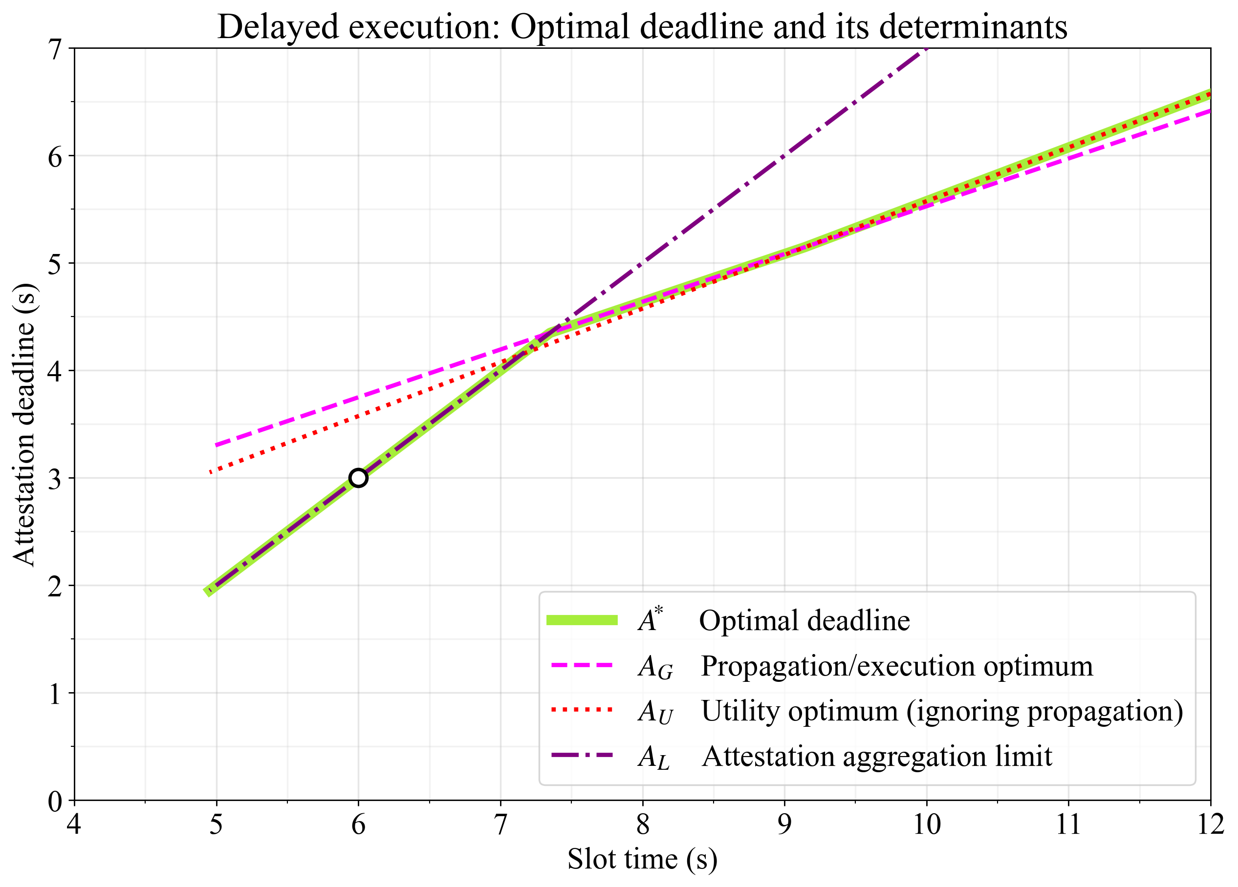
Figure 1. Optimal deadline in delayed execution as the propagation/execution gas optimum A_G, the utility maximum in a purely execution-limited model A_U, and the latest point that allows for attestation aggregation A_L. The circle indicates a potential target at an attestation deadline of 3s in a 6s slot. For optimal throughput, this would require some optimizations to improve propagation time (pushing the optimized lines downward).
With the default constants, the optimal deadline when the slot is 12s long is located at around 6.5s (A_U regime). Below slot times of around 9s, payload propagation time constrains the utility optimum for blobs and execution, making it necessary to compromise by selecting a later attestation deadline (A_G regime). When the slot time falls below around 7.3s, there is no longer enough time for attestation aggregation under A_G, and throughput (propagation) must be compromised by selecting an earlier deadline (A_L regime). It is likely that an implementation of delayed execution under 6s slot times would target the circle at a 3s attestation deadline (as has already been proposed). To achieve a high throughput at 6s, it is then necessary to speed up propagation (pushing down optimized lines in Figure 1) through optimizations such as:
- making call data more expensive,
- improving the p2p layer,
- implementing a multidimensional fee market or macro pricing (to bound worst-case payload sizes).
It can also be assumed that builders themselves may select payload compositions that balance propagation and execution for any given deadline, giving leeway to early deadlines. This will however strain payload propagation for payloads with larger bytesizes. Such payloads may be impossible to get accepted even though they adhere to the gaslimit. This is one of the reasons for why a multidimensional fee market is so attractive.
ePBS
The dual-deadline approach is used when modeling ePBS, allowing for an optimal payload PTC deadline \mathrm{PTC}_P while keeping the PTC DA deadline at the latest possible point of the slot
The payload is released in a trustless setting where the builder in the worst case must release the payload A_d after the attestation deadline. A discussion of the relevance of including A_d in the analysis is offered in Appendix A. The release of blobs is set to c such that the builder does not wait A_d to count attestations before releasing them, allowing slightly longer time for propagation. The attestation deadline is in ePBS set earlier than in delayed execution, specifically at the constant c:
The payload is then released at c+A_d, and inherits its own global latency L_G when propagating as well. The only remaining task is to compute the optimal PTC deadline for the payload, \mathrm{PTC}_P, which is strictly determined as the point that maximizes the total gas, G.
The amount of gas is limited by the execution window, S-\mathrm{PTC}_P, and the execution speed, E_s (gas/s):
It is also limited by the time required to propagate the payload. A payload of gas G takes up to L_G + (G \cdot P_{bg} \cdot L_D) to propagate, and must be allowed to arrive at the latest at the \mathrm{PTC}_P deadline:
This gives the gas constraint on propagation:
The optimal deadline \mathrm{PTC}^*_P is found where the two limits on G are equal:
Solving this for \mathrm{PTC}_P and clamping by \mathrm{PTC}_B yields the final equation:
Once the optimal deadline \mathrm{PTC}^*_P is found, the final throughputs can be determined. The gas per second, G_s, is derived from the propagation constraint:
The blobs per second, B_s, is determined by the time available for blob propagation—from their release at c until the blob deadline \mathrm{PTC}_B, also accounting for their own global latency $L_G$—and the blob rate, B_r:
Figure 2 shows the optimal deadlines for maximizing throughput in ePBS under the baseline constants.
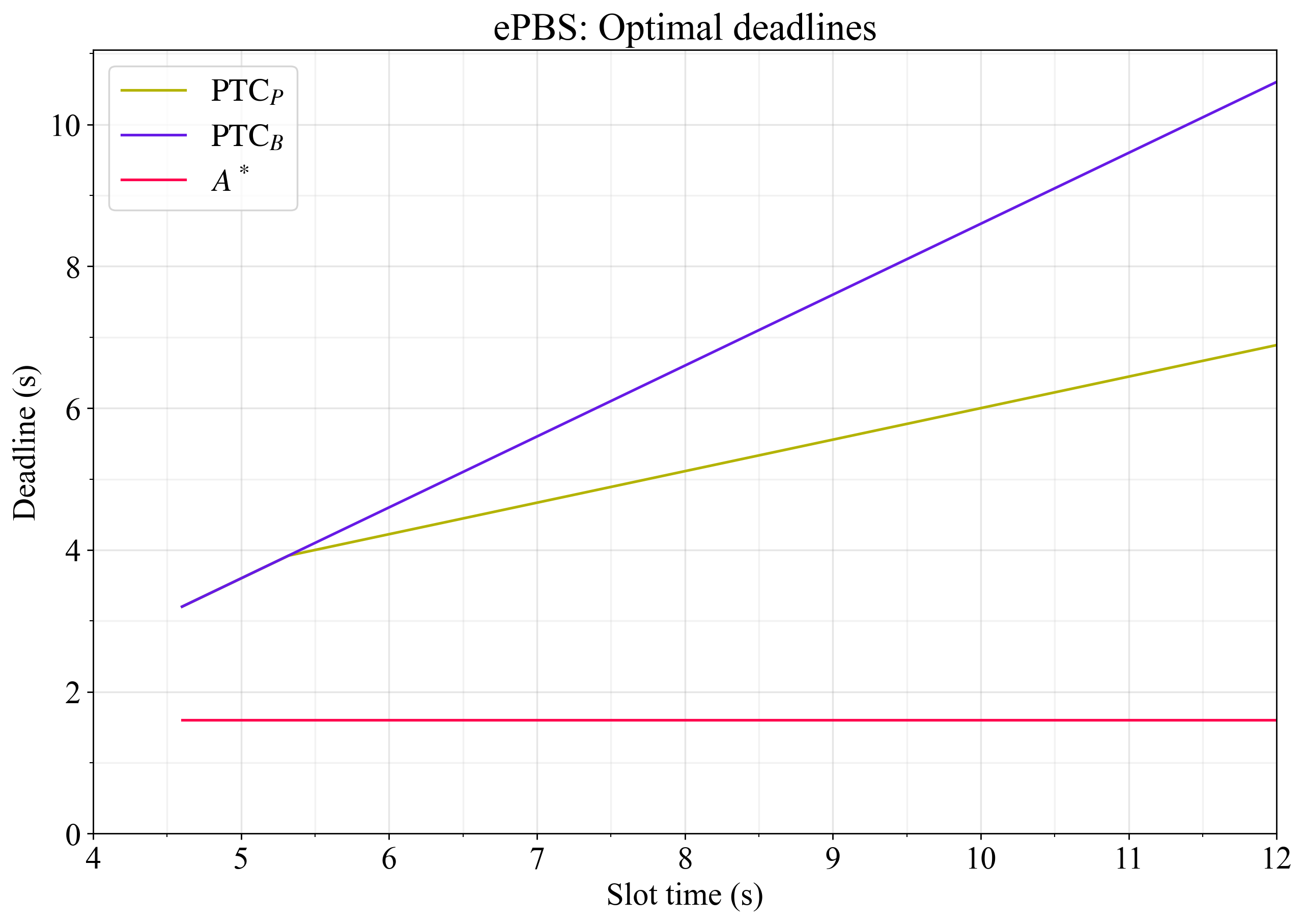
Figure 2. Optimal deadlines for maximizing throughput in ePBS under the baseline constants. The payload observation deadline \mathrm{PTC}^*_P is set at the point that perfectly balances between propagation and execution, adhering to the limit that it cannot happen after the PTC casts its votes at \mathrm{PTC}_B.
Throughput for delayed execution and ePBS
Figure 3 shows execution Mgas/s and blobs/s for delayed execution and ePBS. As evident, ePBS is particularly suitable for scaling blobs, due to the late PTC deadline that it offers. Since the deadline on the payload can be set independently, there is a smooth decay in throughput as the slot time shortens until propagation finally is constrained below 5.5s. Throughput falls smoothly due to the increasing relative importance of:
- the global delay L_G,
- the beacon block propagation time c,
- the time the builder requires for ascertaining that the beacon block will gather enough attestations A_d,
- and the PTC vote propagation time \mathrm{PTC}_d.
Delayed execution is best for scaling L1 gas at longer slot times, since there is L_G-L_R+A_d less delay incurred at the start of the slot and the attestation deadline can be reasonably well balanced between propagation and execution with the default constants. There is then a kink in the throughput curve as the attestation aggregation constraint comes into play at around 7.3s. Throughput falls substantially below this slot length, due to insufficient time for propagation under the baseline constants.
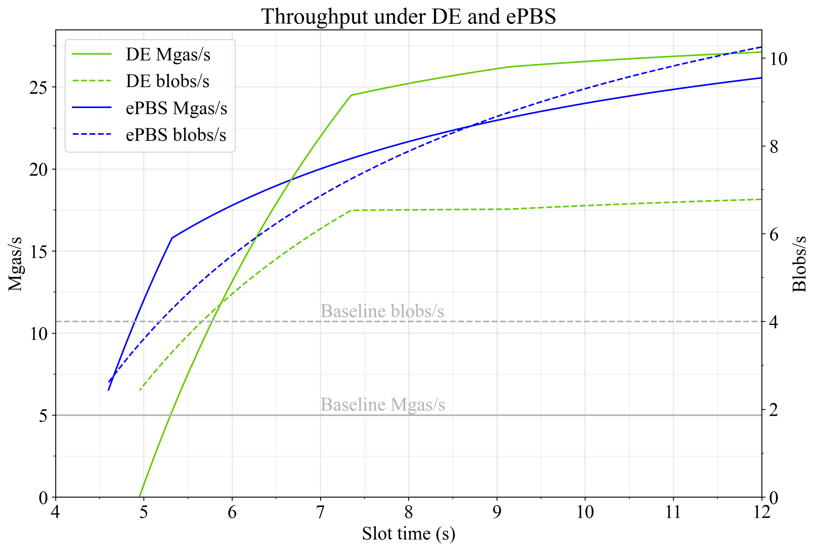
Figure 3. Throughput under delayed execution (green) and ePBS (blue) at different slot times, specified as Mgas/s (full lines) and blobs/s (dashed lines). Both approaches have the potential to scale Ethereum significantly, even at shorter slot times.
Utility according to the Glamsterdam equation
The Glamsterdam equation captures scaling from slot-restructuring, factoring in the relative change in slot time S^* and a subjective scaling factor U_O that captures any additional considerations. Someone may assign U_O>1 to DE if the simplicity of not changing fork choice and not having a PTC is prioritized. If on the other hand, e.g., a trustless payment between builder and proposer is seen as critical, someone may instead assign U_O>1 to ePBS. The full equation is:
The equation also features utility elasticities, which specify the importance of different performance metrics in the utility measure. A utility elasticity of 1 indicates that utility is directly proportional to the metric, while an elasticity of 0 indicates that the metric is irrelevant to overall utility. These elasticities are:
- U_G – The utility elasticity of execution throughput.
- U_B – The utility elasticity of blob throughput.
- U_S – The utility elasticity of shorter slot times.
Figure 4 shows how the utility of delayed execution and ePBS changes across slot time, using the settings U_G=1, U_B=1, U_S=1, and U_O=1. Both restructuring options give about equal utility gains, with DE peaking at 7.3s slot times and ePBS at around 10s slot times.
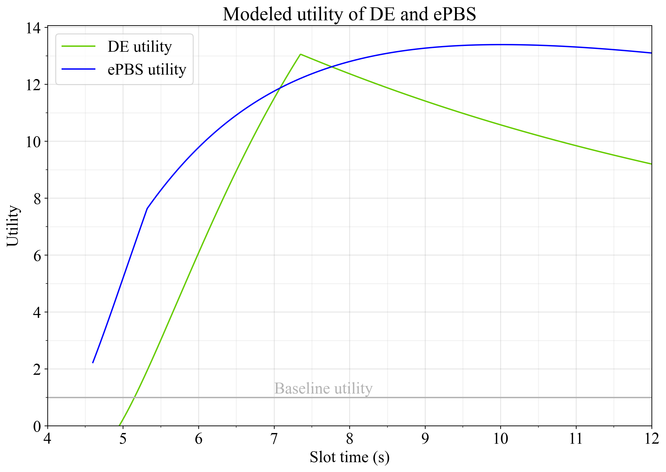
Figure 4. Utility of delayed execution and ePBS when all elasticities are set to 1 and U_O=1 for both options.
We all have different perspectives on which metrics that are the most important, and the elasticities are then useful. For example, given that a target of 32 blobs per slot already is a significant improvement planned for Fusaka and that the current target of 6 blobs is not actually consumed, it may seem reasonable to assign further scaling of blobs a lower importance than scaling of execution gas. Elasticities of U_G=1 and U_B=0.4 capture this notion. Shortening slot times might be assigned somewhere in between in terms of importance, for example U_S=0.7.
Figure 5 shows the outcome with these elasticities, which somewhat favor delayed execution due to the lower assigned importance of blob scaling. On the other hand, some may perceive ePBS as inherently better, due to its ability to facilitate trustless cooperation between builder and proposer. Setting U_O=1.1 for ePBS captures the notion of ePBS being 10% better than delayed execution in terms of non-measurable qualities. The blue dashed line captures this, and utility is maximized either with ePBS at around 9s slot times, or with DE at 7.3s slot times.
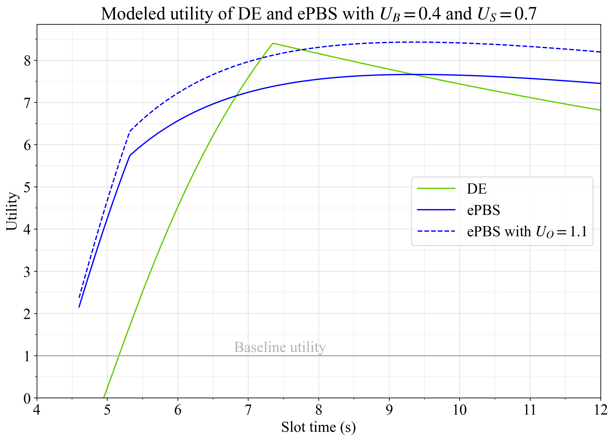
Figure 5. Utility of delayed execution and ePBS with elasticities U_G=1, U_B=0.4 and U_S=0.7. The blue dashed line assigns a subjective benefit of 10% for ePBS over delayed execution (U_O=1.1).
Gas throughput scaling vectors
Main scaling vectors are reviewed in Figure 6, focusing on gas throughput. In this example, the same setting of U_B=0.4 from the previous section was used to allow delayed execution to somewhat prioritize increases in gas throughput over blob throughput when setting the attestation deadline.
The red lines indicate the throughput increase if execution speed doubles from 60M gas/s to 120M gas/s. At long slot times in delayed execution, this greatly improves throughput given that more time can be spent propagating bigger payloads. At shorter slot times, throughput however diminishes just as previously because the then more ideal attestation deadlines A_G and A_U are both impermissible since they would be positioned in the last 3s of the slot (see Figure 1). As a consequence, clients cannot use all available compute cycles. To some extent, it might be possible to account for this, by repricing to substitute propagation for execution, as further outlined in the discussion. In ePBS, the more ideal conditions for attestation propagation means that faster execution is useful at any slot time, overtaking delayed execution in terms of gas throughput already at 8s or shorter slots.
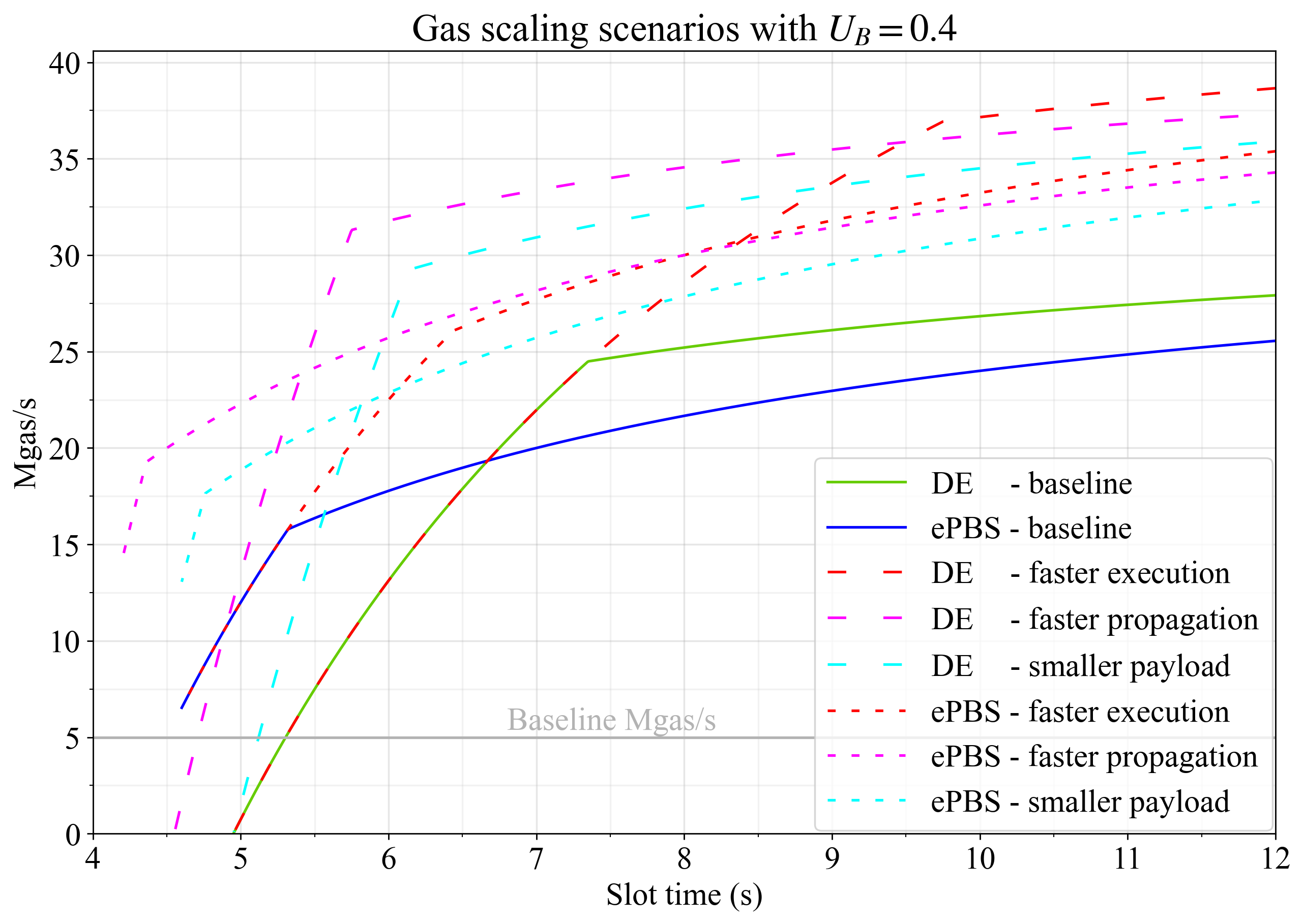
Figure 6. The effect of the main scaling scenarios on gas throughput when setting U_G=1 and U_B=0.4. Faster execution (red), faster propagation (magenta) and smaller payloads (cyan) are analyzed both for DE and ePBS, and compared to baselines.
The magenta lines indicate faster propagation of beacon blocks and execution payloads with the setting L_D=0.4. If U_B=1, i.e., if blob throughput is considered as important as execution throughput, then the magenta line becomes fixed at the green line for longer slot times in delayed execution. This happens because a later deadline allows more blob propagation. When deprioritizing blobs (as in the figure), the attestation deadline can shift earlier and execution throughput can increase. For this reason, fast propagation allows very favorable gas throughput in DE under short slot times, all the way down to 5.7s. For ePBS, there are just as previously steady improvement at all slot times, where \mathrm{PTC}_P always can shift in position to maximize throughput.
The cyan lines indicate smaller payloads, setting P_bg to 0.5 MB per 60M gas. The original setting of 1 MB per 60M gas already assumed some calldata repricing and limiting of the most prominent outliers. This would then need to be pushed further, e.g., making calldata even more expensive.
Figure 7 shows how blob throughput shifts with the improvement to the main scaling vectors. With faster propagation (magenta), ePBS takes advantage of the faster propagation of the beacon block and the earlier attestation deadline to release the blobs earlier. Delayed execution on the other hand takes advantage of faster execution speed (red) allowing for a later attestation deadline at long slot times. Remember that delayed execution must have blobs arrive before the attestation deadline, whereas ePBS might see them instead released around the attestation deadline (among blobs not in the mempool, the builder could potentially release some blobs earlier and may wish to wait to release some until slightly after the deadline).
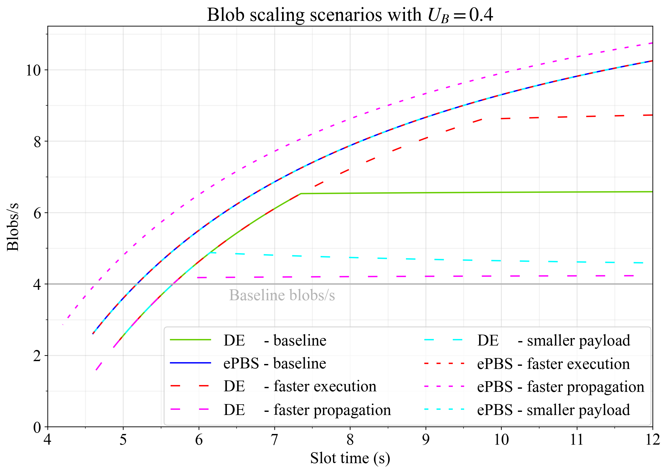
Figure 7. The effect of the main scaling scenarios on blob throughput when setting U_G=1 and U_B=0.4. Faster execution (red), faster propagation (magenta) and smaller payloads (cyan) are analyzed both for DE and ePBS, and compared to baselines.
Much of the improvements for DE in gas throughput for faster propagation and smaller payloads could only be accomplished by shifting the deadline earlier to give more room for execution. This is however detrimental to blob throughput, which therefore falls relative to the DE baseline at the utility maximum, just to accomodate faster throughput. The last section of the post reviews DE with a PTC, where this constraint no longer applies. It is only towards relatively short slot times that faster propagation does improve gas throughput without reducing blob throughput, relative to the DE baseline (as evident in the next utility plot). Overall, ePBS is once again decidedly stronger than DE in terms of blob throughput, at all possible slot times.
Utilities for the scaling vectors were computed using the previously specified elasticities U_G=1, U_B=0.4 and U_S=0.7. The outcome is shown in Figure 8. Fast propagation is a key to achieving a high utility in short slot times for both regimes. It is critical to have the beacon block and payload arrive early in the slot, to leave time for attestation aggregation and execution. For this reason, improvements to the p2p-layer seem important if Ethereum is to scale further. And of course, improvements to attestation aggregation could likewise be useful (the setting of 3s is however already rather optimistic). Figure 9 summarizes the finding by highlighting the winning pipelining option at each slot time, in the different future scaling scenarios.

Figure 8. Utility of the main scaling scenarios when setting U_G=1, U_B=0.4 and U_S=0.7. Faster execution (red), faster propagation (magenta) and smaller payloads (cyan) are analyzed both for DE and ePBS, and compared to baselines.
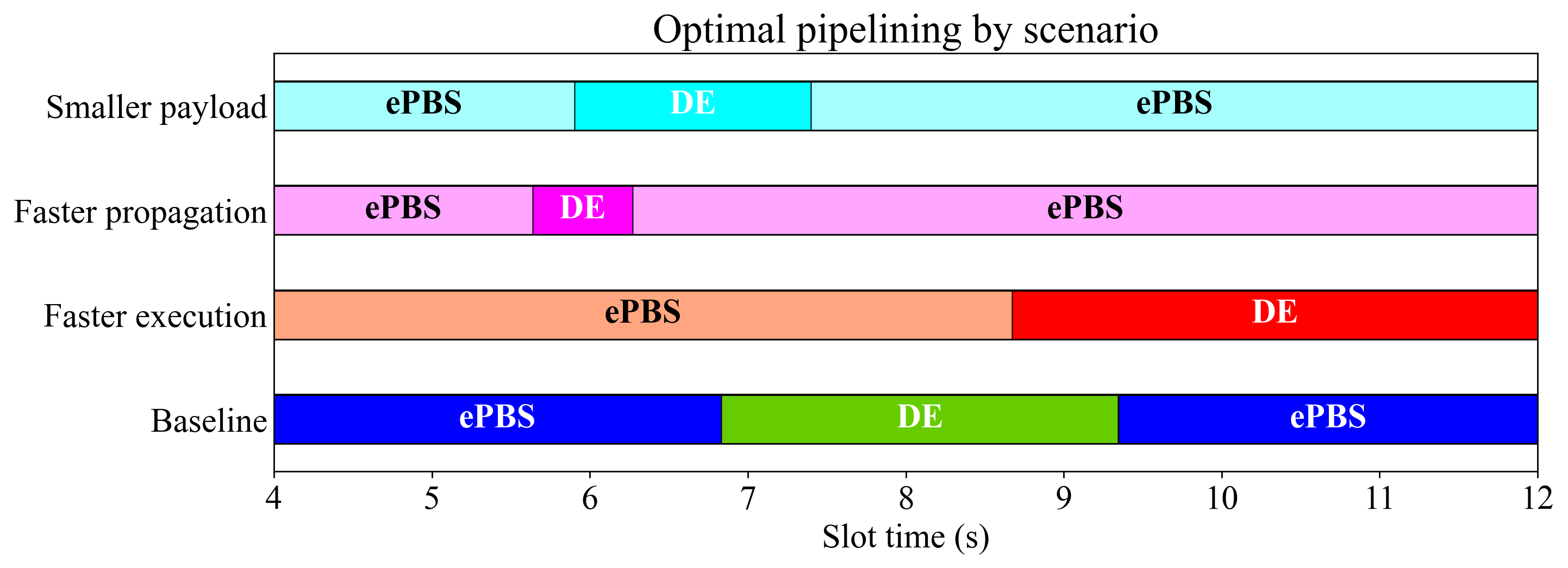
Figure 9. Higher utility between DE and ePBS for the main scaling scenarios when setting U_G=1, U_B=0.4 and U_S=0.7. Faster execution (red), faster propagation (magenta), smaller payloads (cyan), as well as the baselines are visualized.
Alternative scenarios and roadblocks
Figure 10 shows alternative scenarios and roadblocks. A bigger payload of 2 MB per 60M gas is outlined in cyan. Such a payload size is in line with the current worst-case scenarios and would thus be applicable if there is no further data cost increases and we wish to accommodate blocks filled with only calldata (with the effect in the figure also requiring relatively slow propagation, as per the setting L_D=0.8). This would severely reduce throughput, as illustrated in the figure. In this context, we can consider further repricing of data, improvements in propagation speed, or to curtail guarantees on propagation for payloads that contain only calldata. Such payloads can be considered as slightly “artificial” in that they diverge so much from what is considered “normal” usage of blockspace, and that keeping room for such outliers hurt throughput overall. This can then be done either implicitly, by having such a tight deadline that attempts to propagate these payloads may sometimes lead to missed blocks, or explicitly, by limiting this usage pattern with macro pricing or by restricting such payloads altogether.
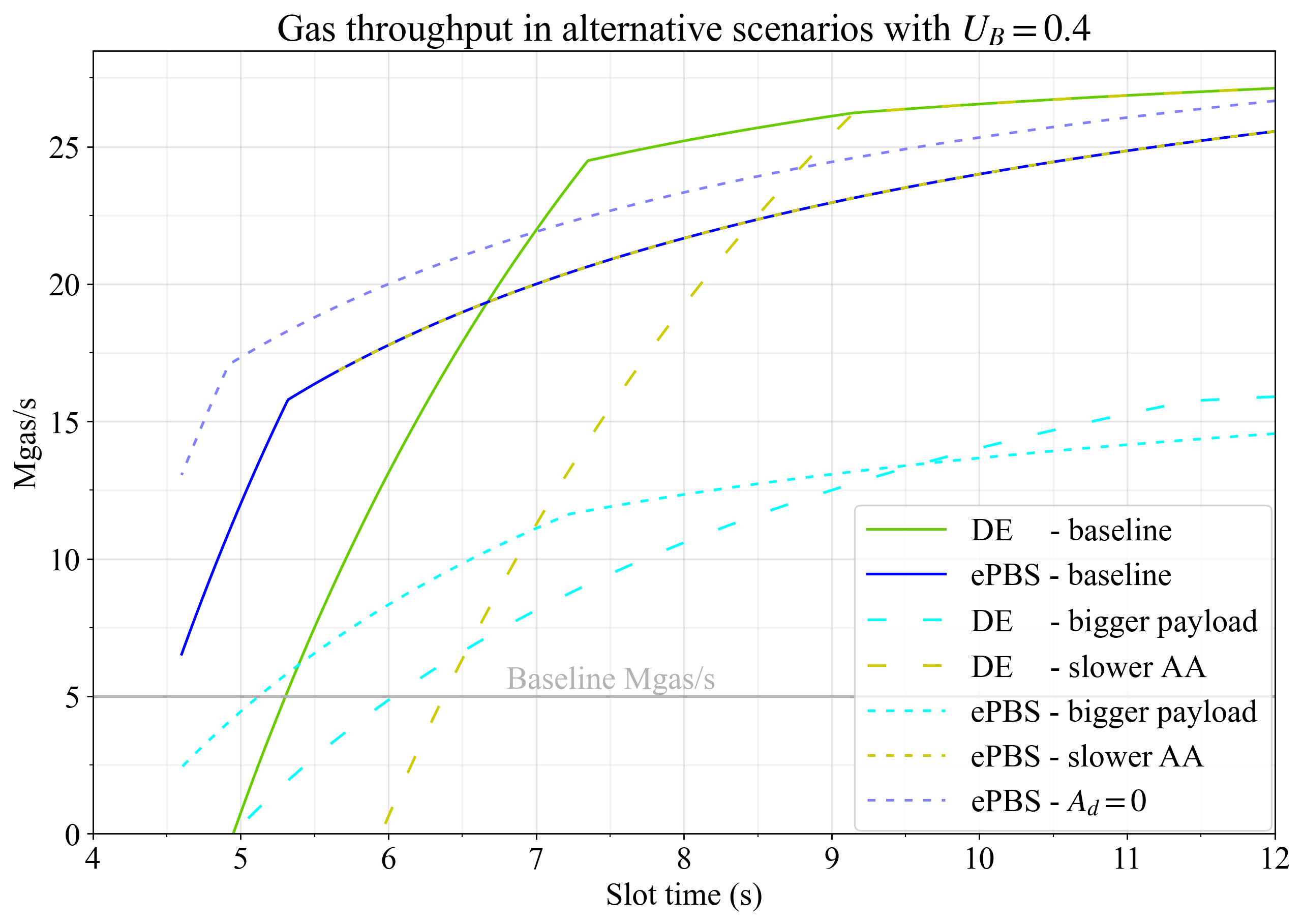
Figure 10. The effect of alternative scenarios on gas throughput when setting U_G=1 and U_B=0.4. Bigger payloads (cyan), slower AA (yellow) and A_d=0 (dashed blue) are analyzed for DE and/or ePBS, and compared to baselines.
The yellow lines show slower attestation aggregation, set at 4s. Once again, we are highlighting a scenario that should perhaps be considered the norm today. Analysis of attestation aggregation has been pointing in various directions over the last month, but it does seem like 4s is much closer to the current status quo than 3s. The speed that can be achieved for attestation aggregation is very important when considering the viability of DE, as shown in the plot. Can we push attestation aggregation down to 3s? If the answer is no, then short slot times seem rather daunting, at least unless we also introduce a PTC in DE. Such a pipelining variant is presented in the next section. As evident, ePBS is not affected negatively by a longer AA, other than making slots below 5.6s impossible.
Finally, the light blue dashed line is ePBS with A_d=0. This is the scenario where the builder always can release the payload at the attestation deadline. In this case throughput increases rather markedly. It is not perfectly clear what the correct setting for A_d is, as discussed in Appendix A.
Figure 11 shows blob throughput in the alternative scenarios and Figure 12 shows the final utility measure. It can be noted that ePBS gives a higher throughput utility than DE at all slot times when builders do not have to take an A_d delay to evaluate attestation propagation.
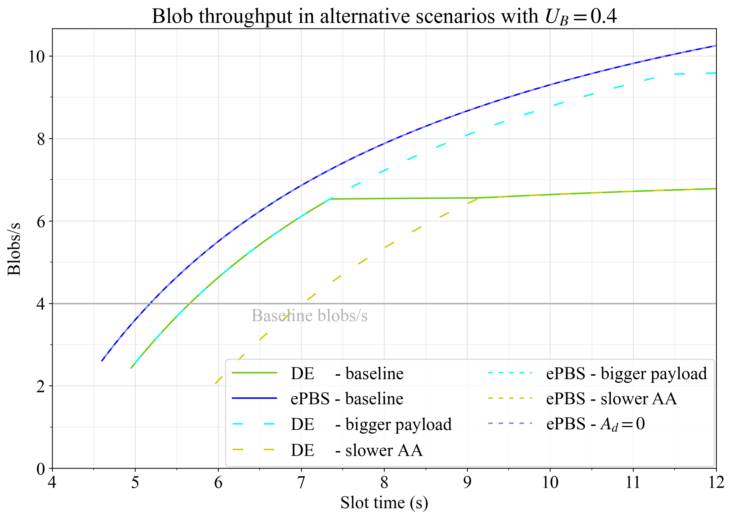
Figure 11. The effect of alternative scenarios on blob throughput when setting U_G=1 and U_B=0.4. Bigger payloads (cyan), slower AA (yellow) and A_d=0 (dashed blue) are analyzed for DE and/or ePBS, and compared to baselines. Neither of these alternative settings however affect blob throughput in ePBS, and they are thus all located overlapping at the blue line.
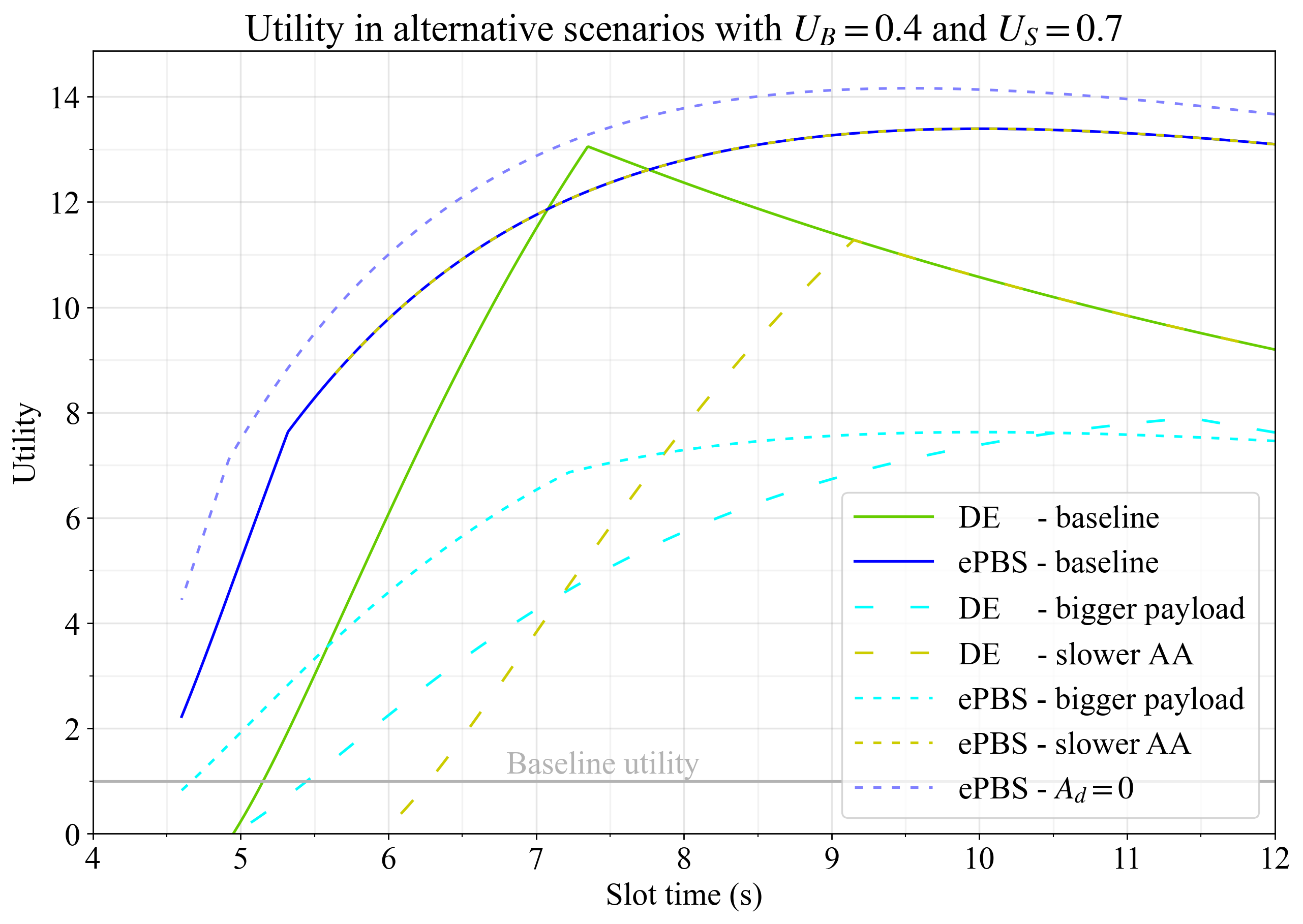
Figure 12. Utility in alternative scenarios when setting U_G=1, U_B=0.4 and U_S=0.7. Bigger payloads (cyan), slower AA (yellow) and A_d=0 (dashed blue) are analyzed for DE and/or ePBS, and compared to baselines.
Alternative pipelining variants
We finally consider alternative specifications. The first is delayed execution that uses a PTC. In this design, the relay releases the beacon block and payload at L_R. The attestation deadline is set as early as possible to allow for attestation aggregation, with the p2p layer instructed to always prioritize propagation of the beacon block such that L_D first only counts against the size of the beacon block and only after that against the size of the payload. The PTC payload deadline \mathrm{PTC}_P is set to maximize throughput and there is no A_d.
While prioritizing the beacon block over the payload enables it to arrive earlier, it seems realistic that this strategy also incurs its own additional delay, such that the average arrival time of the beacon block and the payload is later than if the p2p layer did not have to try to strategize propagation between the two. We model this by adding an additional penalty L_P=0.3 applied to both the beacon block and the payload, by which both arrive later than if they were propagated together (or individually without a priority order, ignoring the effects of variability). The blobs are however released already at L_R and propagate until the PTC deadline at
It is only beneficial to incur the prioritized propagation delay L_P at short slot times where attestation aggregation is a blocker. The plot below therefore uses the optimal propagation strategy, as the option that produces the highest gas throughput. Thus, in the option that prioritizes the beacon block, the attestation deadline is set to
This is as previously subject to the overall feasibility constraint S \ge c + A_a, which ensures there is enough time for attestation aggregation.
Just as in the ePBS model, the total gas, G, is constrained by two conditions, allowing us to find the optimal PTC payload deadline, \mathrm{PTC}_P. The two conditions for G can be set up as the execution constraint
and the propagation constraint, which accounts for the payload arriving after the beacon block at time c
To find the optimal deadline that maximizes throughput, we set these two bounds equal, which gives the equality
Solving this equation for \mathrm{PTC}^*_P yields the final expression:
Once the optimal deadline \mathrm{PTC}^*_P is determined, the final gas throughput G can be calculated by substituting this value back into the propagation constraint:
In the option that does not prioritize beacon block propagation, the attestation deadline and \mathrm{PTC}_P are instead set according to the following condition, where the deadline c itself depends on the resulting gas G:
Combining this condition with the execution constraint and solving for G yields the direct formula for the optimal gas in this scenario:
Should the deadline c derived from this equilibrium gas value be too late for attestation aggregation (i.e., c > S - A_a), the strategy is not discarded. Instead, echoing the A_L clamping logic from the delayed execution model, the deadline is forced to the latest permissible time, A_L = S - A_a. The final gas throughput is then re-calculated as the new bottleneck given by the minimum of the execution and propagation limits at this constrained deadline.
The same analysis used for delayed execution with a PTC can be used for a slot auction ePBS with the auction held before the start of the slot and the fork-choice allowing attesters to vote for an empty payload (beacon block discarded). In this (speculative) design, the relay propagation time can also be removed, by setting L_R=0 in the previous equations.
Figures 13-15 show gas and blob throughput as well as utility with U_G=1, U_B=0.4 and U_S=0.7.

Figure 13. Gas throughput in alternative designs where DE uses a PTC or ePBS uses slot auctions and allows attesters to vote for payloads without beacon blocks.
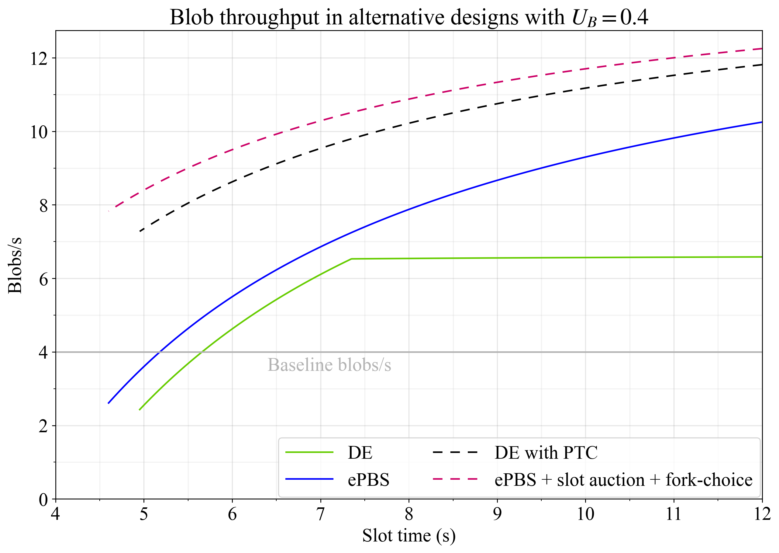
Figure 14. Blob throughput in alternative designs where DE uses a PTC or ePBS uses slot auctions and allows attesters to vote for payloads without beacon blocks.
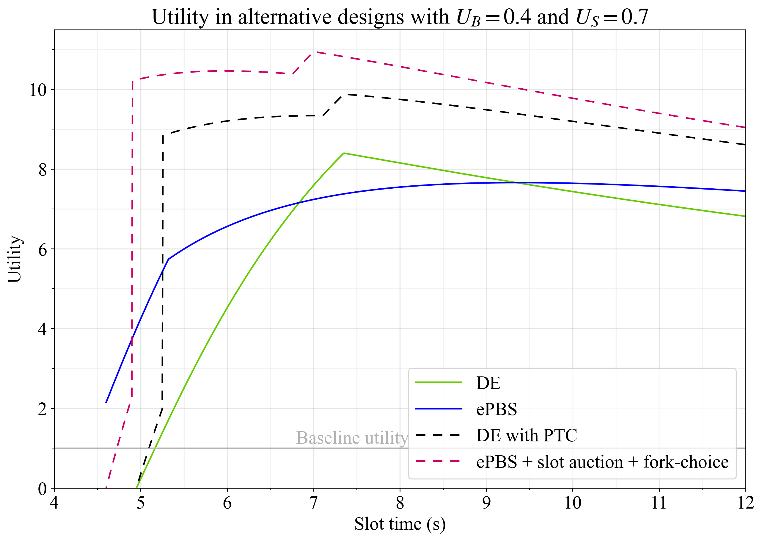
Figure 15. Utility in alternative designs where DE uses a PTC or ePBS uses slot auctions and allows attesters to vote for payloads without beacon blocks, when setting U_G=1, U_B=0.4 and U_S=0.7.
Conclusion and Discussion
Mathematical models of throughput in delayed execution and ePBS have been developed. These models were used to analyze how throughput varies with slot time, relying on basic assumptions when setting the constants. By varying the constants, the impact of further optimizations as well as potential pitfalls were analyzed. Both potential slot reconfigurations lead to significant gains in throughput at short as well as long slot times.
Which configuration to choose is ultimately a question of utility. The Glamsterdam equation models this by assigning utility to each option at all slot times. Due to varying constraints that DE and ePBS must operate under, it is not the case that a specific option is best at every slot time. Generally speaking, ePBS is particularly good at very short and rather long slot times. Delayed execution may oftentimes be better in a window in between, where sufficient time is left for attestation aggregation, and the benefits of an early trustful release of the payload compensates for the absence of the PTC. The execution window must be at least as long as the attestation aggregation time. Under short slot times, the time for payload propagation—relative to the execution window—may then become too short. Of course, the same concern applies to the short time afforded for blob propagation.
A general key concern under short slot times is payload propagation. Improvements to the p2p layer should therefore have high priority. We can of course to some extent substitute time for pricing. Given an increase in execution speed, in the case that a later attestation point is infeasible, we may reprice to prioritize execution. This involves making execution intensive operations less costly and data intensive operations, such as calldata, more costly. From this perspective, an increase in execution speed need not necessarily be wasted if the optimal attestation deadline analytically is pushed into the attestation aggregation region. An analysis of attestation deadlines can thus only take us so far, given the separate toolboxes afforded by the pricing mechanism.
On a similar theme, ceteris paribus, BALs will shift the optimal DE attestation deadline/ePBS PTC payload observation deadline later, assuming that clients have also adopted them. The point is that BALs affect other design parameters. Figure 9 indicated the impact of faster execution, illustrating that this specifically benefits ePBS under short slot times (whereas both options benefit at longer slot times). In the context of BALs, Figure 10, on the other hand, showed that a significant increase in payload size will tend to degrade throughput quite severely (under given assumptions for propagation speed). Thus, maintaining reasonable sizes also for the BAL is worthwhile.
It is finally important to note that the two main design specifications used in this post for DE and ePBS are not the only way to restructure the slot. The last section illustrated further scaling gains when optimizing these constructions, at the cost of additional complexity.
Appendix A
In the trustless exchange of ePBS, the builder cannot count on the proposer to release the beacon block early, such that it quickly gets attested to. The builder must commit to a payload and cannot back out of releasing the exact payload that it committed to when discovering a relatively late release of the beacon block, that just might make it. Furthermore, it must look out for equivocations from the proposer, that may render the payload not included even if released. For this reason, the builder has an incentive to wait a little bit from the attestation time until it releases the payload, and will attach a value in expectation for having the ability to do so.
At bid time, the builder must decide how big a payload it is willing to make, factoring in the worst-case propagation window that it can use. Since the trustless exchange is a block auction, the builder cannot decide the size of its payload after-the-fact, and will be inclined to not make payloads that would put propagation at risk. As a consequence, it should reasonably prefer to build payloads that can propagate sufficiently between A+A_d and \mathrm{PTC}_P.
In the comparison between designs, we fix the payload bytes per gas P_{bg} that we wish to allow builders to build, which together with the gas G gives the upper payload byte size P_{bg}G. Should the deadline be so tight that a payload corresponding to P_{bg} cannot propagate, then builders will naturally adapt by building smaller payloads. But the idea of the analysis of this post is to define the deadlines that allow P_{bg}G to propagate in the analyzed setting. In ePBS, that setting is a trustless exchange. It may indeed seem a bit unfair to only analyze ePBS as a trustless exchange, in that a trustful exchange under ePBS pipelining could produce the highest throughput overall.
It is relevant to mention that in delayed execution, the builder can cancel its bid at the point where it theoretically might be too late for the payload to propagate together with the beacon block. Should we do ePBS as a slot auction instead of a block auction, the analysis will come closer to bid adjustments in delayed execution. The builder can adapt its payload according to its needs, and omitting A_d becomes more intuitive analytically. The builder will still often be able to propagate P_{bg}G if it so wishes, but without taking the same risk. Readers may have different perspectives on these issues, and this post therefore presents the outcome both with and without A_d.