The L2 Fee Vault: Pricing L1 Costs with Feedback Control

[linoscope]

By Lin Oshitani (Nethermind Research) and Ulysse Pavloff (University of Bern).

Thanks to Conor, Ahmad, Gustavo, Daniel, David, and Yuewang for the discussions and/or review.

This work is funded by Taiko as part of the strategic Taiko<>Nethermind partnership.

TL;DR

Pricing L1 posting costs on L2s can be framed as a control problem: a vault tracks the cumulative difference between L2 fee revenue and L1 posting costs, and the L2 fee is the control lever that keeps this vault balanced. Using a simulation driven by historical L1 base/blob fee data, we compare various fee formulas and controller designs for pricing L1 costs on L2s.

Introduction

The Fee Vault Abstraction

Pricing L1 posting costs on L2s can be understood through one core abstraction: a vault. Every L2 transaction pays a fee that flows into the vault, and every time the L2 posts data or proofs to L1, the cost flows out of the vault. The vault balance at any point in time reflects the cumulative difference between L2 revenue collected and L1 costs incurred. In practice, the vault can be a smart contract on L2 that accumulates L2 fees and tracks actual L1 posting costs as they are reported from L1 — see Implementation Notes for how this work.

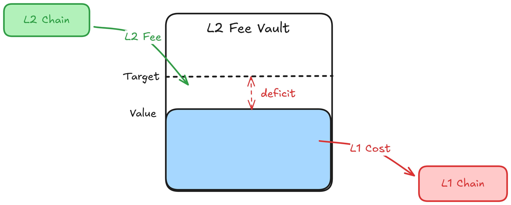
In this framing, a healthy vault — one without a persistent deficit or surplus — means L2 fee revenue and L1 posting costs remain roughly balanced over time. A vault deficit means sequencers are implicitly subsidizing L1 posting costs; a vault surplus means transaction senders are systematically overcharged. The deviation from the vault target therefore provides a natural metric for evaluating fee mechanisms. We use the term vault health to capture this balance; a more precise characterization is given in the section What Makes a Good Fee Mechanism?.

The L2 protocol directly controls the L2 fee it charges users. By adjusting this fee, the protocol can influence the vault balance: raising the fee increases inflow (pushing the vault up), and lowering it reduces inflow (letting the vault drift down). A natural objective is to set the fee such that the vault tracks its target over time, reacting to shifts in L1 costs and L2 demand, while keeping fee volatility low enough that users experience predictable transaction costs.

This framing — a system with a measurable state (vault balance), a target (vault target), and an adjustable input (L2 fee) — is a textbook control theory setting.

Fee vaults (or pools) were originally introduced by Arbitrum in their Fee Pool post. This post extends Arbitrum’s Fee Pool idea in several ways:

1. Frame L2 fee pricing as a general control theory problem.
2. Introduce a feedforward term to enable a unified theory of major L2 fee mechanisms, from OP stack to Arbitrum.
3. Consider the problem in a decentralized sequencer setting.
4. Use a simulation based on historical L1 data to compare controller designs.
5. Document and analyze Arbitrum Nitro’s L1 pricing controller, whose design is not well-documented elsewhere, and compare it against the other approaches in simulation.

Control Theory Analogy: The Thermostat

A classic example in control theory is a thermostat: the room has a current temperature (measured state), a desired temperature (target), a heater whose output can be adjusted (control input), and external factors like weather or open windows (disturbances). The controller reads the temperature, computes the gap from the target, and adjusts heating power to close it.

In summary, for the thermostat:

• Measured state → room temperature
• Target → desired temperature (e.g. 22°C)
• Control input → heater output
• Disturbance → weather, opening windows, etc.

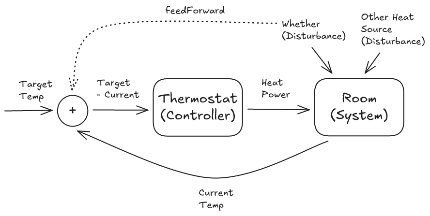
A basic controller reacts only to the gap between the measured state and the target; it waits for the error to appear before correcting. This is feedback: it reacts to the effect of a disturbance after it has already impacted the system. For the thermostat:

• Feedback → Measuring the room temperature and adjusting the heater based on the observed gap from the target temperature.

In contrast, a feedforward term reacts to the cause of a disturbance directly, before the effect propagates through the system. For the thermostat:

• Feedforward → Sensing outdoor temperature or consulting a weather forecast to preemptively adjust the heater output.

Mapping to the Fee Vault

The fee vault maps directly onto this structure:

• Measured state → vault balance
• Target → vault target
• Control input → L2 fee
• Disturbance → L1 base/blob fee fluctuations, L2 demand shifts

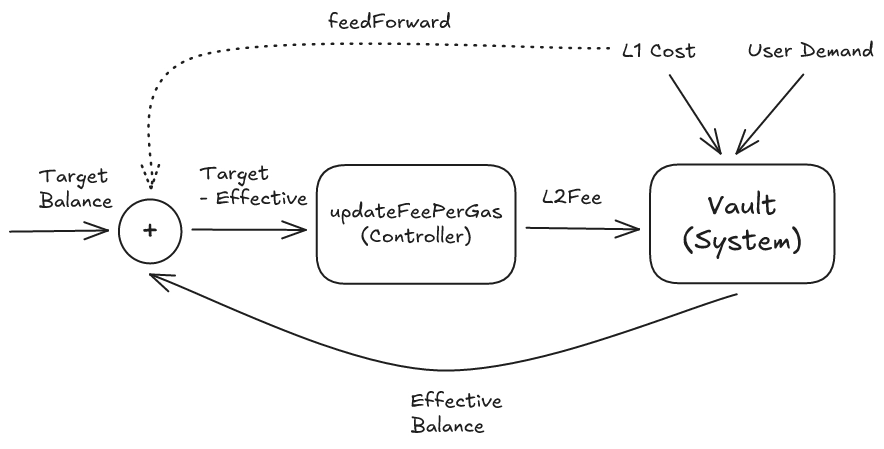
The fee vault controller can use both feedback and feedforward:

• Feedback → Observing the vault balance and adjusting the L2 fee based on the observed gap from the target balance.
• Feedforward → Observing the current L1 base fee and blob fee and factoring them directly into the L2 fee, rather than waiting for the vault balance to drop first.

In fact, in this framework, common L2 fee mechanisms used by chains like Optimism can be viewed as feedforward-only designs. These systems estimate the L1 posting cost for each transaction using the observed L1 base fee and blob base fee at sequencing time and charge users accordingly. In other words, they price L1 data based on an estimate made at sequencing time, rather than the realized posting cost when the batch is actually proposed. On the other hand, they do not maintain a vault or react to cumulative surpluses or deficits. In control-theoretic terms, they pass the disturbance (L1 cost) directly to the fee via the feedforward term, without tracking realized costs in a vault or using feedback from the vault state.

This feedback + feedforward framework can be viewed as a unified framework encompassing all major L2 fee strategies for recovering L1 costs. Pure feedforward (charging each transaction its L1 cost at time of sequencing), pure feedback (fee driven solely by vault deficit), and hybrid designs are all specific cases within the framework.

Note on Decentralized Sequencers

The vault mechanism with feedback control is especially well-suited for rollups with multiple rotating sequencers, such as Taiko’s, for three reasons.

1. It reacts to demand shifts, not just L1 cost changes. Feedforward-only designs are blind to changes in demand on the L2 side. If demand drops, fewer transactions cover the same fixed posting costs, quietly eroding the balance, but the feedforward mechanism won’t notice. A centralized sequencer can mitigate this by waiting until a batch is full before posting, thereby keeping demand largely constant. Rotating sequencers don’t have that luxury: each has a limited window and must post by a deadline, so if demand is low during their window, they post a smaller batch at roughly the same L1 cost, which spikes the cost per transaction. The vault captures this, as demand changes show up as inflow changes — which shows up as degraded vault health — and the controller adjusts the fee in response.
2. It can smooth L1 cost spikes across sequencers. Without a vault, each sequencer bears whatever L1 cost happens during their slot. If one gets hit with a base fee spike, they eat the full cost. With a vault, the protocol can reimburse sequencers from the shared pool, so L1 cost spikes are smoothed over time rather than falling on a single unlucky sequencer. This requires safeguards against reckless posting by sequencers who do not bear the full cost; see [Q1] How do we prevent reckless posting under reimbursement? for details. This makes sequencer economics more predictable and encourages participation even during volatile L1 conditions.
3. It enables incentivized recovery of missed proposals. Suppose a sequencer misses its window to post to L1. Without a vault, the options are either that the missed batch triggers an L2 reorg (bad UX) or that another sequencer recovers it at their own expense with no compensation (bad incentives). A shared vault solves this, as the next sequencer can “recover” the missed batch by posting it alongside its own, and collect the L1 cost part of the fee revenue from the recovered batch as compensation.

What Makes a Good Fee Mechanism?

Before comparing specific fee formulas, it is worth stating explicitly what we want from them. We evaluate mechanisms along two dimensions: vault health and fee volatility.

• Vault health measures how well the mechanism keeps the vault balance near its target over time. A mechanism performs well on this dimension if it avoids deep or persistent deficits and returns toward the target reasonably quickly after a cost shock. A mechanism performs poorly if the vault drifts away from target for long periods, or oscillates without settling.
• Fee volatility measures how abruptly the L2 fee changes from the user’s perspective. Large or frequent jumps make fees less predictable, even when the long-run average remains unchanged.

These objectives are naturally in tension. Mechanisms that react aggressively to keep the vault near target tend to pass shocks through to users more directly, increasing fee volatility. Mechanisms that smooth fees for users tend to absorb shocks in the vault, which can lead to deeper or more persistent deviations from target. The designs studied below occupy different points along this trade-off.

It is worth stressing that in feedforward-only designs, the vault is best understood as an accounting abstraction: it tracks the cumulative difference between fee revenue and realized L1 posting costs. In feedback-based designs, the vault balance becomes part of the control signal used to set fees, and may correspond to an explicit on-chain contract.

Fee Formula Description

Problem Setup

With this control-theoretical framing in place, the central design question is: how exactly should the L2 fee be updated based on the current vault balance and observed L1 costs? Different answers to this question lead to different controller designs. The controllers studied in this paper are built from two conceptually distinct ingredients.

The first is a feedforward term (FF): a direct estimate of the current L1 posting cost, derived from observed L1 base fee and blob fee at sequencing time. FF does not use the vault state at all, it prices the “disturbance” before it hits the vault.

The second is a family of feedback terms, which correct for the gap between the vault balance and its target:

• P (proportional): reacts to the current deficit epsilon(t)
• I (integral): reacts to the accumulated deficit over time
• D (derivative): reacts to how fast the deficit is changing

FF and feedback terms are not of the same nature: FF is a prediction, while P/I/D are corrections. Nevertheless, they can still be treated as modular building blocks: a controller may use them individually, combine several of them, or mix feedforward and feedback terms. The mechanisms studied here are illustrative combinations within this broader design space: FF-only, P-only, PI (proportional + integral), P+FF, and the Arbitrum-style controller which is best understood as PD (proportional + derivative).

Assumptions and scope:

• Inelastic demand. We treat demand as inelastic throughout — under some fee cap, higher fees always increase vault inflow. If demand is elastic, controllers can become unstable: a fee hike that drives users away deepens the deficit instead of closing it. See [Q3] What if the fee gets too high and drives users away? for mitigations.
• L1 cost only. This post focuses on the L1 cost side of L2 fees. L2 congestion pricing (adjusting fees based on L2 block utilization) is an orthogonal concern that can be layered on top independently, since congestion pricing responds to L2 utilization whereas the vault controller responds to the L1 cost gap.
• Abstracted per-transaction data accounting. In practice, each transaction’s share of the L1 posting cost depends on how much data it contributes to the batch being posted. Throughout this post, we abstract away this per-transaction data accounting and treat F(t) as a fee per data unit.

Notation

Common variables:

• t: current time step (i.e., block timestamp)
• F(t): the L2 fee charged at time t (the controller’s output)
• V(t): vault value at time t
• V_target: target vault value
• delay: observation delay in L1 blocks (in Taiko terms, the anchoring lag — how far the currently anchored L1 block trails the latest L1 head)
• epsilon(t): normalized deficit ratio at time t, defined as (V_target - V(t - delay)) / V_target
• F_min: minimum allowed fee
• F_max: maximum allowed fee
• FeeRange: fee range, defined as F_max - F_min
• clamp(x, lo, hi): restricts x to the range [lo, hi] — if x is below lo it returns lo, if above hi it returns hi, otherwise x itself

Simulation Setup

All simulations in this post are driven by 365 days of historical Ethereum mainnet base fee and blob base fee data (2025-02-06 through 2026-02-06), shown below:

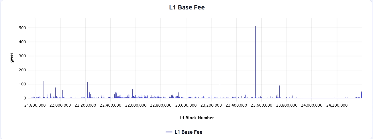
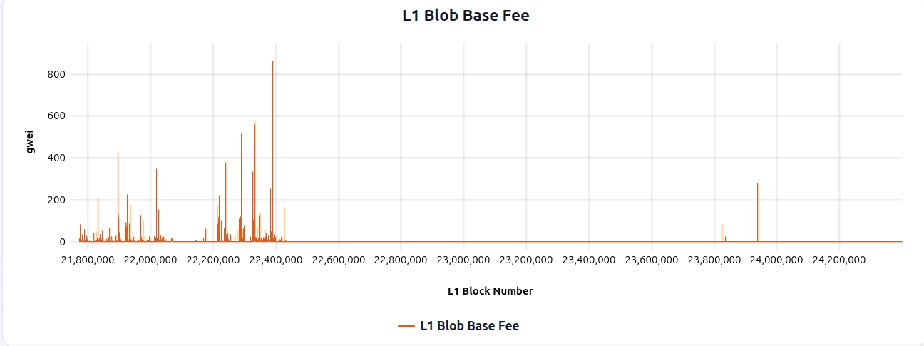
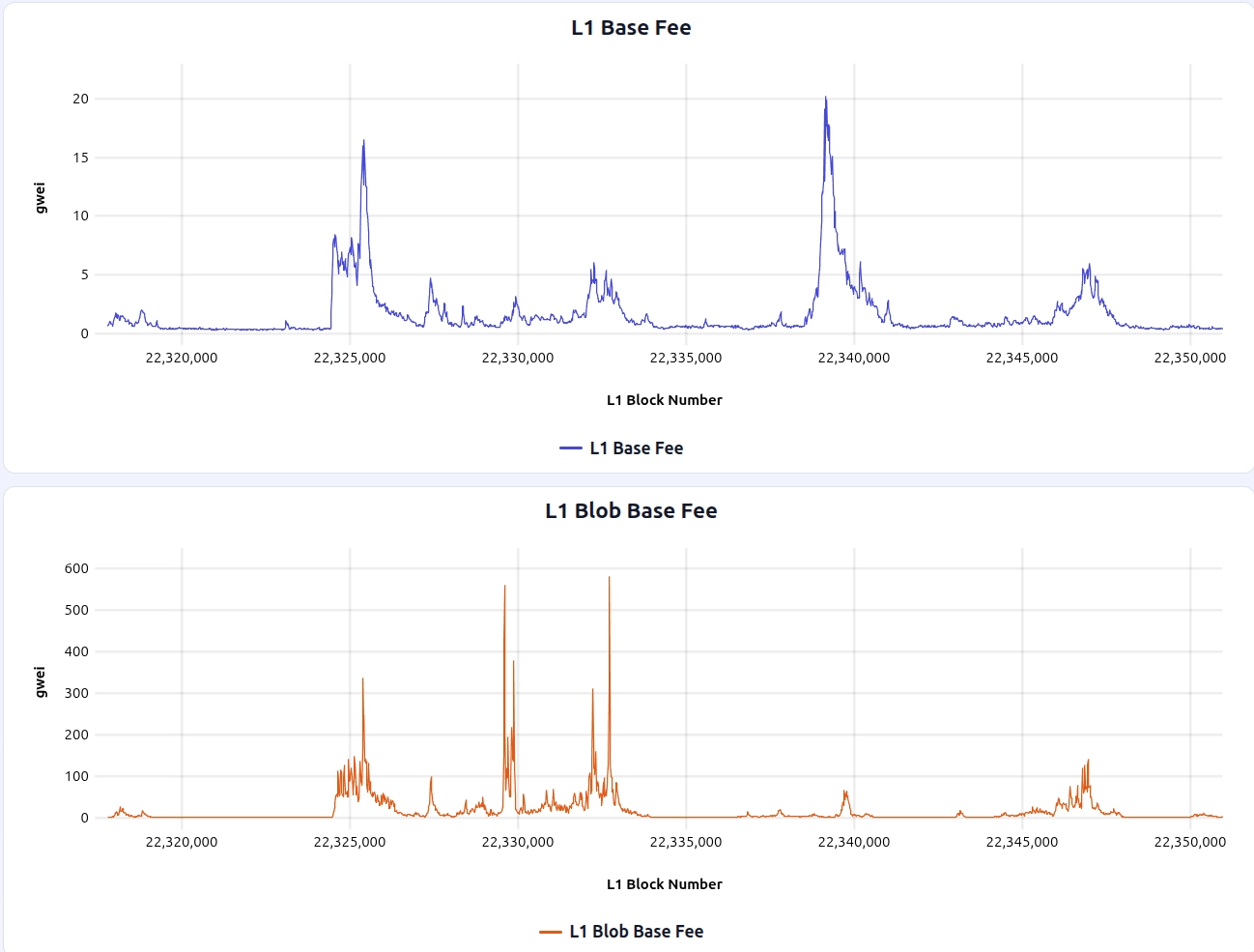
This window includes a notable blob fee spike around L1 block 22389679, which can be useful to zoom in on when comparing how different fee mechanisms react to spikes:

Key simulation parameters:

• Data posting frequency: every 10 L1 blocks
• L2 TPS: 1 tx/s
• Vault target: 10 ETH
• Fee range: 0.01–1 Gwei

These parameters are chosen to be broadly realistic and illustrative, rather than calibrated to a specific deployment. The L1 fee data and controller simulations can be explored interactively in this simulator UI.

Feedforward-only (FF-only)

The feedforward-only approach is the most widely deployed approach today, and is used by Optimism and other major L2s. The idea is to estimate the L1 posting cost at sequencing time and charge it directly to the user, with no vault or feedback loop. In control-theoretic terms, this is pure feedforward: the controller observes the L1 cost (disturbance) and prices it into the fee before it materializes as an actual posting cost.

The formula is as follows:

• BaseFee(t), BlobFee(t): the L1 execution base fee and blob base fee at time t.
• alpha_gas, alpha_blob: scaling weights that convert L1 gas and blob costs into the per-L2-transaction share.

FF(t) = alpha_gas * BaseFee(t - delay)
      + alpha_blob * BlobFee(t - delay)

F(t)  = FF(t)

The delay parameter here reflects a trust/latency trade-off. Chains with a trusted sequencer (such as Optimism) can push the latest L1 base fee and blob fee into L2 via an oracle, effectively operating with delay ≈ 0. A trustless alternative is to import L1 state via the chain’s native L1→L2 messaging path (e.g., Taiko’s anchor transaction or Arbitrum’s delayed inbox), which avoids the trust assumption on an oracle but introduces an observation delay of several L1 blocks.

Simulation & Analysis

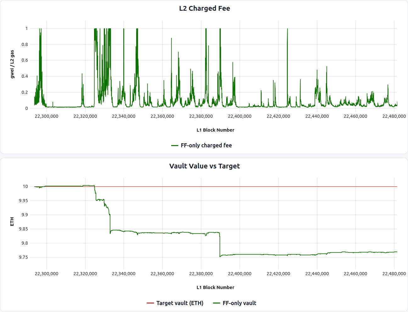
Although FF-only does not use the vault as an input, we still track the implied vault balance in simulation as an evaluation metric. The results are as follows (can be seen interactively through UI here):

Pros/cons of this approach are:

Pros:

• The vault tracks its target well during periods when the fee has room to adjust — i.e., when it isn’t capped at the maximum.

Cons:

• FF-only also exposes L2 users directly to L1 fee volatility. Although we assume inelastic demand in this post for simplicity, fee spikes that are exogenous to L2 demand can hit users especially hard when willingness to pay has not increased, making demand effectively more elastic and increasing the risk of choking L2 activity during L1 spikes (in contrast with demand-driven spikes, where willingness to pay is typically higher). See [Q2] How much should L2 fees be isolated from L1 fee fluctuations? for details on whether and how to smooth this.
• FF-only prices current L1 conditions, but cannot repair accumulated misses. These mainly arise from F_max clipping during large L1 spikes. Once the spike passes, there is no feedback term to push the vault back toward its target.

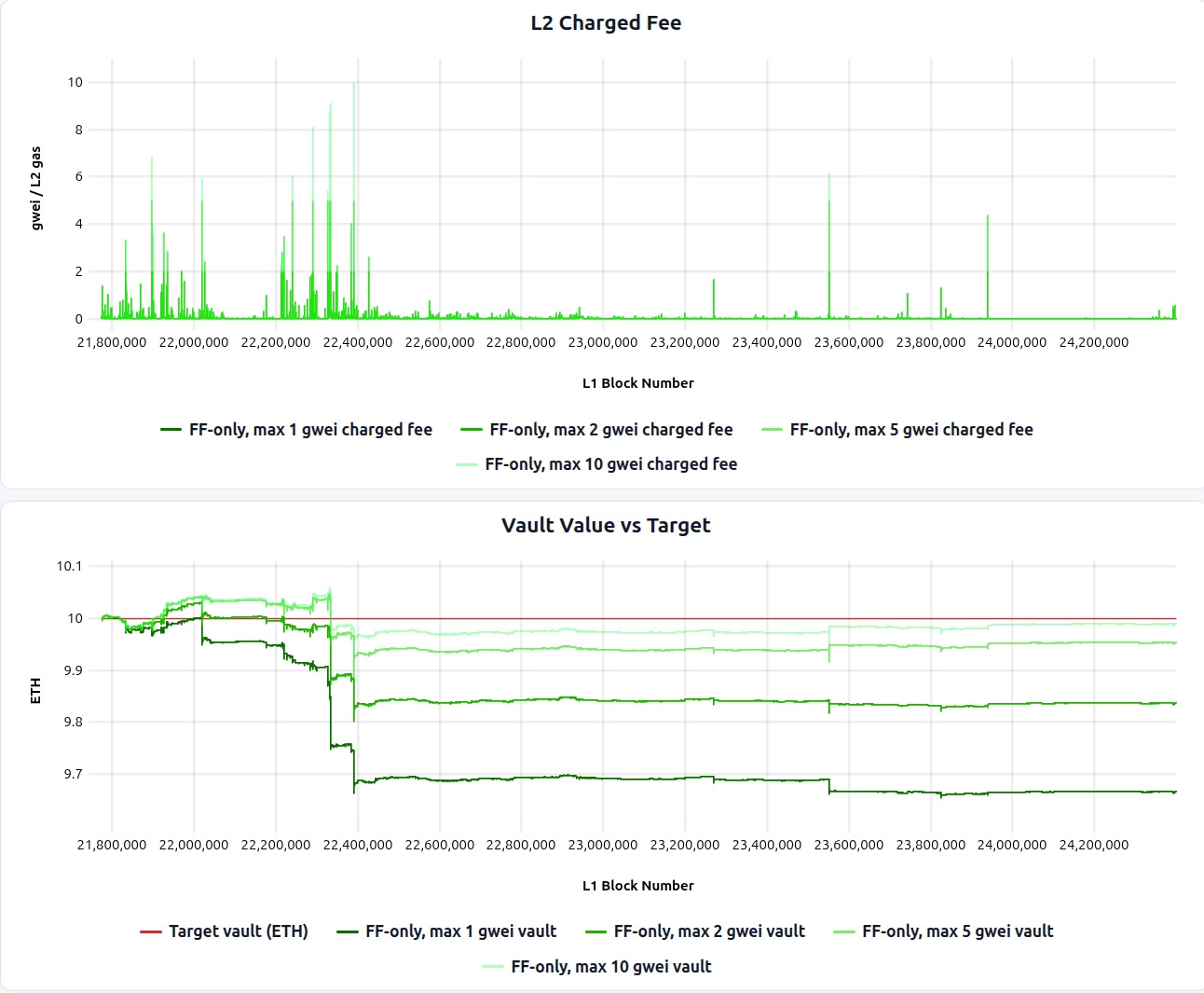
The F_max sweep below makes this trade-off especially clear (simulation link). Raising F_max from 1 gwei to 2, 5, and 10 gwei materially improves vault health, because fewer L1 spikes are clipped and more of the realized posting cost is passed through to users. But this comes at the cost of significantly higher fee volatility:

P-controller (P-only)

The P-controller sets the fee directly from the current vault deficit: the further the vault is below target, the higher the fee, and vice versa. The trade-off is that if the vault settles at a persistent small deficit, the P-controller applies the same small correction indefinitely without escalating, leaving the vault slightly below target. (steady-state bias).

• Kp (proportional gain): controls how aggressively the fee reacts to the current deficit. Higher Kp means a stronger correction per unit of deficit.

The formula is as follows:

P(t) = Kp * epsilon(t) * FeeRange
F(t) = clamp(P(t), F_min, F_max)

Simulation & Analysis

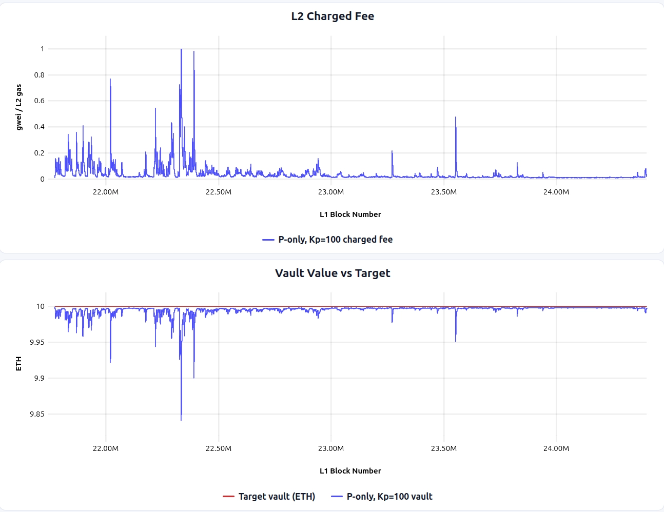
The results are shown below (simulation link). The first plot shows the L2 fee charged by the controller over time, and the second plot shows the vault balance trajectory. The red line marks the target, and the blue line tracks the actual vault value (a downward move indicates a growing deficit).

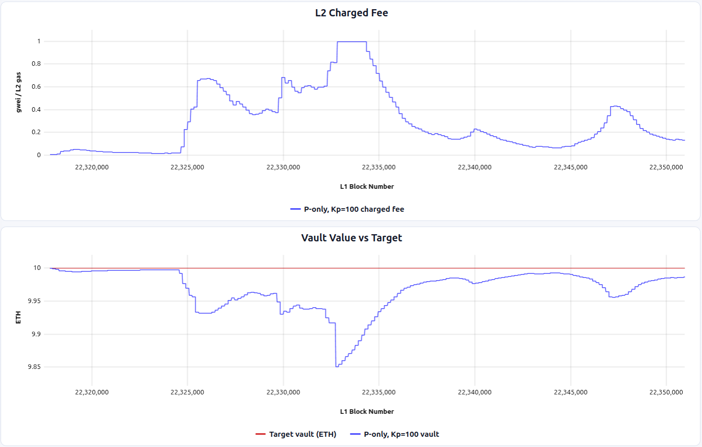
When zoomed in around the blob fee spike:

Pros/cons of this approach are:

Pros:

• Compared with FF-only, the P-controller delivers low fee volatility because it responds to accumulated vault error instead of passing each L1 cost spike straight through.
• It can restore vault health over time. After a shock, the fee stays elevated until the vault recovers, rather than dropping immediately once the L1 spike passes.

Cons:

• The controller is purely reactive, so abrupt it takes time until sudden L1 cost spikes get reflected into the L2 fee.
• It has a steady-state bias: once the vault is slightly below target, the controller can settle into a slightly elevated fee that keeps the vault near, but not exactly at, the target.

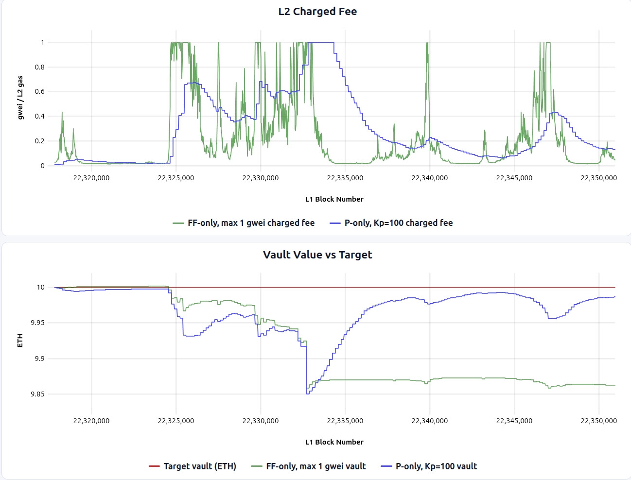
This trade-off is especially clear around the blob-fee spike near L1 block 22389679, as shown below compared with FF-only (simulation link). Blue line is P-only, while green line is FF-only, capped at 1 gwei.

PI controller

A common way to address the steady-state bias of a P-controller is to add an integral term. The integral accumulates the deficit signal over time, so if the vault sits below target for long enough, the controller applies a progressively stronger correction until the bias is removed.

• Ki (integral gain): controls how aggressively the fee ramps up in response to a persistent deficit.
• I_acc(t) (integral accumulator): the running sum of the deficit signal.
• I_min, I_max: bounds on the integral state (for anti-windup).

The formula is as follows:

I_acc(t)  = clamp(I_acc(t-1) + epsilon(t), I_min, I_max)

P(t)      = Kp * epsilon(t) * FeeRange
I(t)      = Ki * I_acc(t) * FeeRange

F(t)      = clamp(P(t) + I(t), F_min, F_max)

Simulation & Analysis

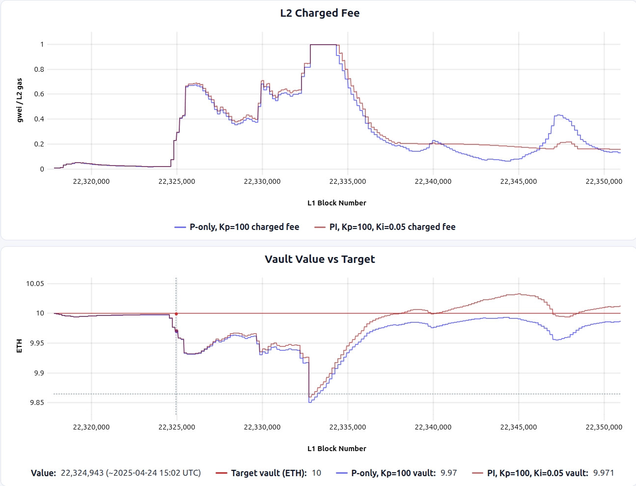
The results are shown below, blue is P-only and brown is PI controller.

And if we zoom into a blob fee spike timeframe:

Pros/cons of PI-controller is:

Pros:

• PI addresses the P-controller’s steady-state bias: if the vault sits below target for long enough, the integral term accumulates and pushes the fee high enough to close the remaining gap.
• After extended deficit periods, PI tends to recover faster than P-only, since the integral term retains “memory” of the persistent error.

Cons:

• The integral term can create overshoot: after conditions normalize (e.g., after an L1 spike passes), the accumulated integral can keep the fee elevated, temporarily pushing the vault above target, which increases fee volatility from the users’ perspective.
• PI introduces additional tuning complexity (choice of Ki and anti-windup bounds). Poor tuning can cause oscillations or slow convergence.

P + Feedforward (P+FF)

P+FF is one example of combining feedforward and feedback terms in a single controller. Here, the feedforward term prices observed L1 conditions into the fee immediately, while the proportional term still corrects any residual vault deficit.

FF(t) = alpha_gas * BaseFee(t - delay)
      + alpha_blob * BlobFee(t - delay)

P(t)  = Kp * epsilon(t) * FeeRange          // same proportional term as above
F(t)  = clamp(FF(t) + P(t), F_min, F_max)

Simulation & Analysis

P+FF is best to evaluate with direct comparison against P-only around the blob-fee spike, where the trade-off is most visible:

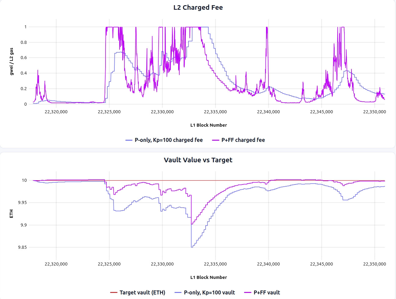
Pros/cons of this approach are:

Pros:

• It keeps the vault closer to target than P-only, because part of the expected L1 cost is priced in before the posting cost actually hits the vault.

Cons:

• It passes much more L1 volatility directly through to users, producing higher fee volatility than P-only.

In practice, the vault-health improvement over P-only is modest in this simulation, which makes it questionable if it’s worth the added fee fluctuation.

Arbitrum-style controller

The controllers above react only to the vault balance’s position relative to the target. Arbitrum Nitro’s L1 pricing controller also reacts to how fast the gap is changing and in what direction. On top of the “proportional” signal, it takes the “derivative” of the vault value. In that sense, it is best thought of as a PD-like controller.

• F(t): effective fee level after update t
• U(t): data units consumed in the posting interval (in Nitro: compressed calldata bytes × 16)
• EquilUnits: the equilibration horizon, i.e. how many data units to work off the current surplus. Larger values mean gentler correction.
• Inertia: sets the dampening midpoint. InertiaUnits = EquilUnits / Inertia is the interval size at which half the correction applies.

InertiaUnits       = EquilUnits / Inertia
desiredSlope(t)    = -S(t) / EquilUnits
actualSlope(t)     = (S(t) - S(t-1)) / U(t)
slopeCorrection(t) = desiredSlope(t) - actualSlope(t)
feeChange(t)       = slopeCorrection(t) * U(t) / (InertiaUnits + U(t))
F(t+1)             = max(0, F(t) + feeChange(t))

The controller works in terms of surplus S(t) = V(t) - V_target (note the sign flip from the deficit epsilon(t) used above) and updates an effective fee F(t) incrementally after each posting event. Based on the current surplus, it computes a desiredSlope, the rate at which surplus needs to change to return to zero within EquilUnits worth of posted data. When an L1 batch posting happens, it computes the actualSlope, how surplus actually changed per data unit. The fee is adjusted based on the gap: slopeCorrection = desiredSlope - actualSlope.

However, actualSlope is noisy, especially when few data units were consumed (small U(t)). To prevent overreacting, the correction is scaled by U(t) / (InertiaUnits + U(t)): when U(t) is small, most of the correction is suppressed; when large, most applies; when U(t) = InertiaUnits, exactly half applies.

Simulation & Analysis

The plots below compare Arbitrum-style with P-only around the blob-fee spike (simulation link):

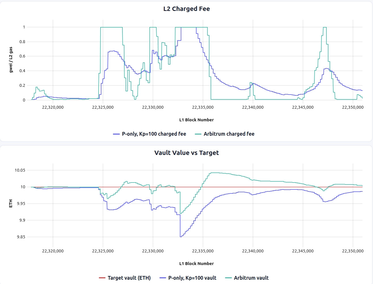
Pros:

• It achieves better vault health than P-only in the spike window, with shallower drawdowns.
• Fee volatility is much lower than FF-only.

Cons:

• Fee volatility is higher than under P-only; the fee repeatedly snaps between low and high values, rather than following P-only’s smoother hump-shaped path.
• The controller is harder to reason about and tune than a plain P-controller, because the behavior depends on the interaction between EquilUnits, Inertia, posting cadence, and interval size U(t).

Simulations Takeaways

The simulations point to a consistent trade-off: better vault health usually comes at the cost of higher fee volatility.

• P-controller offers the lowest fee volatility but moderate vault health in these simulations, while also recovering deficits over time. Its main weakness is that vault health recovery is not the fastest, and it takes time to react to sudden L1 cost spikes.
• Arbitrum-style achieves stronger vault health at the cost of higher fee volatility than P-only, especially around sharp stress events like the L1 cost spike, but it has more jagged fee updates and higher complexity.
• FF-only can track realized L1 costs well when the fee has sufficient headroom (i.e., F_max is high enough that spikes are not clipped), but it passes L1 volatility directly through to users. And if fees are capped at F_max during large spikes, it cannot recover the missed revenue afterward because there is no feedback term to push the vault back toward target.
• P+FF improves vault health relative to P-only, but in this simulation, the gain is modest compared with the UX cost from feeding more L1 volatility directly into the fee.
• PI-controller improves steady-state tracking versus P-only, but can introduce overshoot and more user-facing fee fluctuation.

Overall, the simulations suggest that, if L2 fee fluctuation is a concern, the main design choice is between P-only and Arbitrum-style: P-only if fee smoothness, implementation simplicity, and predictability are the priority; Arbitrum-style if tighter target tracking is worth accepting noisier fees and a more complex controller. While PI reduces steady-state bias, it tends to overshoot, and tuning complexity makes it less compelling, especially when the steady-state bias of P-only is within a tolerable range.

It is worth noting that the controllers explored here represent only a small slice of a vast design space. Many other controller architectures, including other variations of PID controllers, adaptive-gain schemes, and hybrid designs that blend feedback and feedforward in different proportions, remain unexplored and are left to future work.

Implementation Notes

In practice, the L1 posting cost has to be imported from L1 to L2 to be accounted in the vault, which lives in the L2. The high-level flow is:

1. Record L1 cost on L1. When a sequencer posts L2 data or proofs to L1, the L1 inbox contract records the actual posting cost (gas used × base fee, blob count × blob fee).
2. Import into L2 via L1→L2 messaging. The recorded cost is passed to the L2 fee vault contract via the chain’s L1→L2 message-passing mechanism. In Taiko’s case, this happens via the anchor transaction — each L2 block includes an anchor that imports the latest L1 state, including any newly recorded posting costs. Arbitrum uses the delayed inbox mechanism.
3. Update vault balance and compute fee. The fee vault on L2 debits the imported cost from its balance, yielding the updated V(t). The controller then uses this balance to compute the next L2 fee F(t).

This means the vault’s view of L1 costs is inherently delayed. It can only reflect costs that have been recorded on L1 and imported into L2. This delay is captured by the delay parameter in the controller formulas above.

Open Questions

[Q1] How do we prevent reckless posting under reimbursement?

As discussed in Note on Decentralized Sequencers, the vault can reimburse sequencers for their L1 posting costs. But this creates a potential moral hazard: sequencers might post too frequently (small, inefficient batches), fail to time their posts to avoid L1 fee spikes, or overpay for priority fees — since the vault absorbs the cost anyway.

Mitigations to consider:

• Use a fixed priority fee in the reimbursement formula, or do not consider priority fee at all. This caps what the vault will cover — if a sequencer overpays on priority fees, they bear the excess themselves.
• Cap reimbursement below 100% (e.g., 90%) when a sequencer posts at a loss. This keeps sequencers incentivized to post cost-efficiently, since they always have some skin in the game.

[Q2] How much should L2 fees be isolated from L1 fee fluctuations?

Any controller with a feedforward component (FF-only, P+FF) passes L1 base fee and blob fee volatility directly into the L2 fee. This volatility is exogenous to L2 demand. On L1, fee spikes are demand-driven, so the users causing the congestion are the ones paying, and higher fees don’t necessarily choke activity. On L2, the situation is different: an L1 cost spike (e.g., from a token sale on L1) raises L2 fees without any corresponding increase in L2 willingness to pay. Because L2 users have no reason to value the spike, demand elasticity is steeper, increasing the risk of choking L2 activity.

This raises a design question: should the vault deliberately absorb short-term L1 spikes to reduce fee volatility, or pass them through for tighter vault health?

[Q3] What if the fee gets too high and drives users away?

All controllers above assume that a higher fee leads to greater vault inflows within some capped fee limit (F_max). But in practice, if the fee climbs too high, users stop transacting, and the drop in volume can more than cancel out the higher per-transaction fee. This can create a death spiral: high fee → fewer transactions → deeper deficit → even higher fee.

Mitigations already in place:

• F_max clamp: all controllers enforce a hard fee ceiling, which is the main guard against pushing fees too high.

Under the assumption that F_max is low enough not to drive away significant demand, the current simulations hold. But this remains an assumption, and if F_max sits above the point where demand becomes elastic, the controllers could still enter the “death spiral” described above.

Additional mitigations to consider:

• Simulate with an assumed demand elasticity curve: Run the controller simulation under a model in which transaction volume declines as fees rise, to test robustness beyond the inelastic regime.
• Monitor and react to demand shifts: track rolling L2 gas usage and automatically soften fee increases when volume drops quickly after a fee increase.