Data availability sampling (DA-sampling or DAS) today is planned to be done with KZG commitments. KZG commitments have the advantage that they are very easy to work with, and have some really nice algebraic properties:
- An evaluation proof has constant size and can be verified in constant time.
- There exists an algorithm to compute all proofs evaluating a deg < N polynomial at each of N roots-of-unity in O(N * log(N)) time.
- You can linearly combine commitments to get a commitment of the linear combination: com(P) + com(Q) = com(P + Q)
- You can linearly combine proofs: Proof(P, x) + Proof(Q, x) + Proof(P + Q, x)
The first is a nice efficiency guarantee. The second ensures that producing a blob that can be DA-sampled is easy: if it takes O(N^2) time to generate all proofs, then it would require either highly centralized actors or a complicated distributed algorithm to make it DAS-ready.
The third and the fourth are very valuable for 2D sampling, and enabling distributed block producers and efficient self-healing:
- A block producer only needs to know the original M commitments to “extend the columns” with an FFT-over-the-curve and generate 2M commitments that are on the same deg < M polynomial.
- You can do not only per-row reconstruction but also per-column reconstruction: if some values and proofs on a column are missing (but more than half are still available), you can do an FFT to recover the missing values and proofs.
However, KZG has a weakness: it relies on complicated pairing cryptography, and on a trusted setup. Pairings have been understood for over 20 years, and the trusted setup is a 1-of-N trust assumption with N being hundreds of participants, so the risk in practice is high and this author believes that proceeding with KZG is perfectly acceptable. However, it is worth asking the question: if we don’t want to pay the costs of KZG, can we use inner product arguments (IPAs) instead?
See the first half of this article for an explainer of IPAs.
IPAs have the following properties:
- An evaluation proof has logarithmic size and can be verified in linear time (roughly 40ms for a size-4096 polynomial)
- There is no known efficient multi-proof generation algorithm.
- Commitments are elliptic curve points and you can linearly combine them just like KZG commitments
- There is no known way to linearly combine proofs.
Hence, we keep some properties and we lose some. In fact, we lose enough that our “current approach” to generating, distributing and self-healing proofs is no longer possible. This post describes an alternative approach that, while somewhat more clunky, still achieves the goals.
An alternative approach
First, instead of generating 2N independent proofs for a deg < N polynomial, we generate a proof tree. This looks as follows:
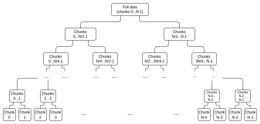
We interpret the data in evaluation form, treating it as a vector: [x_0, x_1 ... x_{2N-1}], where the polynomial P = \sum_i x_i L_i (where L_i is the deg < 2N polynomial that equals 1 at coordinate i and 0 at the other coordinates in the set).
Each node in the tree is a commitment to that portion of the data, along with a proof that that commitment actually “stays within bounds”. For example, the \frac{N}{2} ... N-1 node would contain a commitment C_{[\frac{N}{2}, N-1]} = x_{\frac{N}{2}}L_{\frac{N}{2}} + x_{\frac{N}{2} + 1}L_{\frac{N}{2} + 1} + ... + x_{N-1}L_{N-1}. There would be an IPA proof that C_{[\frac{N}{2}, N-1]} actually is a linear combination of those points and no other points.
We generate two trees, the first for [x_0 ... x_{N-1}] and the second for [x_N ... x_{2N-1}], and the “full” commitment to a piece of data consists of C_{[0,N-1]} and C_{[N,2N-1]}.
To prove a particular value x_i, we simply provide a list of (sub-commitment, proof) pairs covering the entire range 0...N-1 or N....2N-1 (whichever contains i), excluding i, as well as a proof that the top-level commitment that i is not part of was constructed correctly. For example, if N = 8 and i = 3, the proof would consist of C_{[0,1]}, C_{2}, C_{[4,7]} and their proofs, as well as a proof that C_{[8,15]} was constructed correctly. The proof would be verified by verifying the individual proofs and checking that the commitments add up to the full commitment.
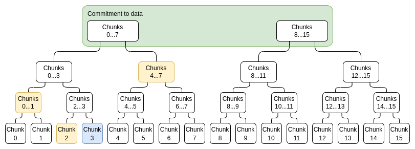
Blue: chunk 3, yellow: proof for chunk 3.
Note that to improve efficiency, each chunk does not need to be a single evaluation; instead, we can crop the tree so that eg. a chunk is a set of 16 evaluations. Given the combined size of the proofs will be larger than this regardless, we lose little from making chunks larger like this.
Generating these proofs takes O(N * log(N)) time. Verifying a proof takes O(N) time, but note that verification of many proofs can be batched: the O(N) step of verifying an IPA is an elliptic curve linear combination, and we can check many of these with a random linear combination. O(N) field operations per proof would still be required, but this takes <1 ms.
Extension: fanout greater than 2
Instead of having a fanout of 2 at each step, we can have a higher fanout, eg. 8. Instead of one proof per commitment, we would have 7 proofs per commitment. At the bottom level, for example, we would have a proof of \{1,2,3,4,5,6,7\}, \{0,2,3,4,5,6,7\}, \{0,1,3,4,5,6,7\}, etc. This increases total proof generation effort by \approx \frac{7 * \frac{7}{4}}{3} x (7 proofs per node, each proof 1.75x the size of the original, but 3x fewer layers, so ~4.08x more effort total), but it reduces proof size by 3x.
Proof size numbers
Suppose that we are dealing with N = 128 chunks of size 32 (so we have deg < 4096 polynomials), and a fanout of (4x, 4x, 8x). A single branch proof would consist of 3 IPAs, of total size 2 * (7 + 9 + 12) = 56 curve points (~1792 bytes) plus 512 bytes for the chunk. This compares to 48 byte proofs for a 256 byte or 512 byte chunk today.
Generating the proofs would require a total of 2 * 8192 * (3 * 2 + 7) curve multiplications (3 * 2 for the two fanout-4 layers and 7 for the fanout-8 layer), or a total of ~212992 multiplications. Hence, this would require either a powerful computer to do quickly (a regular computer can do one multiplication in ~50 us, so this would take 10 seconds which is a little too long) or a distributed process where different nodes focus on generating proofs for different chunks.
Verifying the proofs is easy, as proof verification can be batched and only a single elliptic curve multiplication done. Hence, it should not be much slower than with KZG proofs.
Self-healing
Self-healing could not effectively be done column-by-column. But can we avoid requiring a single healer to have all of the data (all 2N chunks from each of all 2M polynomials)?
Suppose that a single row is entirely missing. It’s easy to use any column to reconstruct the value in the missing row in that column. But how to prove it?
The simplest technique is cryptoeconomic: anyone can simply post a bond claiming a value, and someone can later take that claim together with a branch proof proving a different value to slash that validator. As long as enough legitimate claims are available, someone on that row subnet can combine together the claims and reconstruct the commitment and the proofs. Validators could even be required to publish such claims for sample indices that they are assigned to.
A cryptoeconomics-free but more technically complicated and slow alternative is to pass along M branch proofs for values along that column, along with a Halo-style proof that the proofs verify correctly.