AirScript: language for defining zk-STARKs

This follows up on my earlier post genSTARK: a JavaScript zk-STARK generation framework.

I’ve implemented a first prototype of a simple language for writing AIR constraints for zk-STARKs. The language is called AirScript. The new version (v0.4) of genSTARK library, which I just released, now relies on AirScript for STARK definitions.

Here is an example of how a MiMC STARK can be defined using AirScript:

define MiMC over prime field (2^256 - 351 * 2^32 + 1) {

    transition 1 register in 2^13 steps {
        out: $r0^3 + $k0;
    }

    enforce 1 constraint of degree 3 {
        out: $n0 - ($r0^3 + $k0);
    }

    using 1 readonly register {
        $k0: repeat [...]; // actual 64 constants go between the brackets
    }
}

And here is AirScript for a modified version of Rescue hash function:

define Rescue over prime field (2^64 - 21 * 2^30 + 1) {

    alpha: 3;
    inv_alpha: 0-6148914683720324437;

    MDS: [
        [18446744051160973310, 18446744051160973301],
        [                   4,                   13]
    ];

    INV_MDS: [
        [ 2049638227906774814,  6148914683720324439],
        [16397105823254198500, 12297829367440648875]
    ];

    transition 2 registers in 32 steps {
        S: [$r0, $r1];
        K1: [$k0, $k1];
        K2: [$k2, $k3];
        S: MDS # S^alpha + K1;
        out: MDS # S^(inv_alpha) + K2;
    }

    enforce 2 constraints of degree 3 {
        S: [$r0, $r1];
        N: [$n0, $n1];
        K1: [$k0, $k1];
        K2: [$k2, $k3];

        T1: MDS # S^alpha + K1;
        T2: (INV_MDS # (N - K2))^alpha;

        out: T1 - T2;
    }

    using 4 readonly registers {
        $k0: repeat [...]; // actual 32 constants go between the brackets
        $k1: repeat [...]; // actual 32 constants go between the brackets
        $k2: repeat [...]; // actual 32 constants go between the brackets
        $k3: repeat [...]; // actual 32 constants go between the brackets
    }
}

You can see complete exmaples of these STARKs here.

Input injection

v0.4 of genSTARK library also supports Input injection. This basically allows aggregating proofs of the same computation for different inputs into a single proof.

For example, we could aggregate proofs of knowledge of Rescue hash preimage for 16 values into a single proof. The resulting proof is ~114 KB in size (while a proof for a single value is ~37 KB in size). You can see more benchmarks here.

Future plans

AirScript is not yet expressive enough to support easy definitions of more complex STARKs. For example, defining a STARK that could prove membership of a value in a Merkle tree is rather cumbersome. This is something I’m planning to address next.

If you have any thoughts or feedback on these, let me know!

8 Likes

To improve expressivity one possible direction is to create an N-variable opcode-based language, something as follows:

  • You choose N, the number of state variables
  • You choose K, the number of opcodes. You define what each opcode does, in the form S_next[i] = formula(S_prev[1] ... S_prev[n]) (or more generally, formula(S_prev[1] ... S_prev[n], S_next[1], S_next[n]) to allow fast verification of inverse functions), where formula is a low-degree polynomial in the given N or 2N variables
  • You provide zero or more readonly registers as before
  • You provide log(K) readonly registers code that expresses in binary form which opcode to execute at each step. The actual constraints enforced then become:
    • code[i] * (1 - code[i]) = 0 (each code item is zero or one)
    • (1 - code[0]) * (1 - code[1]) * ... * (1 - code[log(K)]) * opcode_constraint[0](...) = 0 (either the opcode is not 0 or constraint 0 is satisfied)
    • code[0] * (1 - code[1]) * ... * (1 - code[log(K)]) * opcode_constraint[0](...) = 0 (either the opcode is not 1 or constraint 1 is satisfied)

This would make expressing programs of the form “do this, then do that, then do this other thing” much easier to express; potentially the Merkle proof example I gave in the other thread could be done inside of it. The only thing not fully generic about this approach is that verification scales linearly for anything that requires more than a few state registers (you could simulate many registers with one register by treating the one register as a state root and updating it by showing Merkle branches, but that incurs high overhead…)

I had a similar idea of how it would work in the background - but I’m hoping to come up with language constructs that would make it even easier to reason about the “foreground”.

For example, for “do this, then do that” scenario, I’m considering something like this:

transition 4 registers in 32 steps {
	for 31 steps do {
		// compute values for all 4 registers
	}

	for 1 step do {
		// compute values for all 4 registers
	}
}

In the background the construct could be very similar to what you are describing: there would be an “implied” readonly register (e.g. $c0) with value 1 for the first 31 steps and value 0 for the last step. Then the statements in the first for block will be multiplied by $c0, and the statements in the second for block would be multiplied by 1 - $c0.

This could potentially be extended to something like this:

transition 4 registers in 32 steps {
	for 31 steps
		with [$r0, $r1] do {
			// compute values for the first 2 registers
		},
		with [$r2, $r3] do {
			// compute values for the other 2 registers
		};

	for 1 step do {
		// compute values for all 4 registers
	}
}

And maybe even result in something that would allow AIR “reusability” like this:

transition 4 registers in 32 steps {
	for 31 steps
		with [$r0, $r1] do RescueHash,
		with [$r2, $r3] do RescueHash;

	for 1 step do {
		// compute values for all 4 registers
	}
}

There are still a lot of moving parts though and I’m not sure if the exact definition as I outlined above would work best. So, I might have to come up with some other construct that would work better.

The main problem I see with that approach is that the bulk of code that I expect people will want to write in the long term is not going to be these long repeats, but rather the operation is going to change step by step. So making for x steps do y be the base construct makes everything needlessly verbose. IMO the ideal goal would be a language similar to “normal” languages, something like:

for i in range(32):
    r1 <- r1**3 + c1[i]
r2 <- r1 + 5
r3 <- RescueHash(r1, r2)
r4 <- r3 + 10
for i in range(32):
    r4 <- RescueHash(r4, c2[i])*c3[i] + RescueHash(c2[i], r4)*(1 - c3[i])
....

This gets us to something that regular people could easily program in :slight_smile:

Yep - something like that is the ultimate goal, but getting there will take some time :slight_smile:

At this point, I’d like to keep it somewhat close to the actual execution semantics, ideally, with each block of statements describing a single state transition. But even with this restriction, the syntax can be simplified when verbosity adds no extra information.

The thing that seems more complicated to me is coming up with elegant constructs to loop over multiple sets of inputs. For example, for a Merkle proof of depth 16 there would be 16 input values to hash sequentially. This can be handled using readonly registers, but this approach is not very intuitive. Once I come up with a good way to address this, other things should fall into place as well.

Readonly registers seems like the logical place to put that. The goal would be that a slightly higher level language would see code such as:

for i in range(32):
    r4 <- RescueHash(r4, c2[i])*c3[i] + RescueHash(c2[i], r4)*(1 - c3[i])

And if you specify c = [....] as an input then it would automatically place that into the right position of the readonly registers.

Is the language I suggested above really that far away? It seems to be that if you wrap every line in for 1 step do { ... } (and the for i in range(32) becomes for 32 steps do { ... } where i can be determined from a computational step counter register) then you basically convert it to the language you suggest above.

I don’t think it’s that far away - but my mind works slowly in these things - so, just taking it one step at a time.

While I’m still thinking about looping constructs, I came up with a set of minimal changes needed to allow relatively straightforward script for Merkle proofs. Below is an example of how a transition function could look like for a Merkle proof of depth 16 (transition constraints would look not too differently):

transition 8 registers in 16*32 steps {
    when ($k0) {
        // constants for Rescue hash
        K1: [$k1, $k2, $k3, $k4];
        K2: [$k5, $k6, $k7, $k8];

        // transition for hash($r0,$r1)
        S1: [$r0, $r1, $r2, $r3];
        S1: MDS # S1^alpha + K1;
        S1: MDS # S1^(inv_alpha) + K2;

        // transition for hash($r4,$r5)
        S2: [$r4, $r5, $r6, $r7];
        S2: MDS # S2^alpha + K1;
        S2: MDS # S2^(inv_alpha) + K2;
        
        out: [...S1, ...S2];
    }
    else {
        // this would happen every 32nd step

        h: $k9 ? $r0 | $r4;
        S1: [h, $k10, 0, 0];
        S2: [$k10, h, 0, 0];
        
        out: [...S1, ...S2];
    }
}

Here is a brief explanation:

when…else

when ... else is a new construct (not yet implemented). Basically, it means that out values in the when clause are multiplied by $k0, while out values in the else clause are multiplied by 1 - $k0. In the Merkle proof case, $k0 would be a readonly register with 32 repeated constants such that the first 31 values are 1, and the last value is 0. This effectively means that when clause gets executed for 31 steps, and else clause gets executed for 1 step, and then the whole thing loops around.

Rescue hash

In this implementation, Rescue hash requires 4 registers. The first two registers hold 2 values to be hashed, and the other 2 registers are “working” registers needed for internal calculations (they are initialized to 0’s). The output of the hash (after 31 steps) is in the first register. In the above example, $r0 and $r5 would be initialized to the leaf value for which the proof is created, while $r1 and $r4 would be initialized to the value of its sibling.

Vector concatenation

[...S1,...S2] is a way to concatenate 2 vectors. It is not yet implemented, but I’ve created an issue for it already.

Conditional expression

$k9 ? $r0 | $r4 basically reduces to $r0 * $k9 + $r4 * (1 - $k9). This is not yet implemented but I have an issue for it as well. The purpose of this statement is to select a hash from $r0 or from $r4 based on the value in $k9. In the Merkle proof case, $k9 would contain a binary representation of the leaf’s index for which the proof was created. For example, if the proof is for index 5, the binary representation would be 0000000000000101, which means that values in $k9 would be 1 for steps 0 and 64, and 0 for all other steps.

Also, in the above example $k10 would be a readonly register with hashes of sibling nodes for each level of Merkle proof.

While when...else construct is pretty powerful (and can be easily nested), I don’t think it’s the best approach long-term. I think a looping construct would be more powerful and extensible - but I’m still working on that.

Definitely an improvement! I do feel like moving toward figuring out the right way to implement code that does different things at each line of code (is that just a log-n-depth tree of nested when/else statements?) is the big challenge.

I’ve just released an updated version of the library. It now includes support for many new AirScript features which make it fairly easy to write transition functions and constraints for something like a Merkle proof. Here is a high-level list of new features in this release:

  • Public and secret input registers - this allows defining readonly registers without any values. The values for such registers are provided at the time of proof generation and/or verification.
  • Binary registers - these are registers which are limited to holding 0 or 1 (relevant for conditional expressions).
  • Conditional expressions - this includes ternary operator and when..else statements.
  • Vector composition - this provides a simple syntax for combining multiple vectors together.
  • Constraint degree inference - the degree of transition constraints are now inferred automatically based on underlying arithmetic expressions. So, there is no need to specify the degrees manually.

Using these features, I wrote up a STARK for verifying Merkle proofs (based on Rescue hash function). Here is the transition function in AirScript and I also have a more detailed explanation here and the actual STARK is here.

transition 8 registers in 8*32 steps {
    when ($k0) {
        // constants for the hash function
        K1: [$k1, $k2, $k3, $k4];
        K2: [$k5, $k6, $k7, $k8];

        // compute hash(p, v)
        S1: [$r0, $r1, $r2, $r3];
        S1: MDS # S1^alpha + K1;
        S1: MDS # S1^(inv_alpha) + K2;

        // compute hash(v, p)
        S2: [$r4, $r5, $r6, $r7];
        S2: MDS # S2^alpha + K1;
        S2: MDS # S2^(inv_alpha) + K2;

        out: [...S1, ...S2];
    }
    else {
        // this happens every 32nd step

        // select the hash to move to the next step
        h: $p0 ? $r4 | $r0;

        // set values for p and v for the next step
        S1: [h, $s0, 0, 0];
        S2: [$s0, h, 0, 0];

        out: [...S1, ...S2];
    }
}

In terms of performance, a proof for Merkle branch verification is 114 KB for a tree of depth 8, and 136 KB for a tree of depth 16. The proofs take 0.8 and 1.6 seconds to generate respectively. I have some more benchmarks here.

1 Like

Not sure I’m understanding what’s going on here.

when ($k0) {

The idea here is that $k0 is a constant register which is set to 0 for steps that are multiples of 32 and 1 elsewhere, correct?

       S1: [$r0, $r1, $r2, $r3];
       S1: MDS # S1^alpha + K1;
       S1: MDS # S1^(inv_alpha) + K2;

What does it mean for S1 to be set to three different things? Also, is “#” a comment or something else?

   h: $p0 ? $r4 | $r0;

So $p0 is a list of bit constants that states what the path in the Merkle tree is?

       S1: [h, $s0, 0, 0];
       S2: [$s0, h, 0, 0];

Where are these values being read? It seems like they’re just being overwritten above…

And where are the constraints on the input and output?

Here are quick answers to the questions, but I’ll also write up a separate post later to explain in detail how this all works.

  1. Yes, $k0 is a constant register that repeats the following pattern every 32 steps: 31 ones followed by 1 zero. So, for steps 0-30 $k0=1 and for step 31 $k0=0; then for steps 32-62 again $k0=1 and for step 63 $k0=0 etc. This pattern is defined on line 131 of this file.
  2. # is a matrix multiplication operator. I describe all available operators here.
  3. S1 is just a variable - so, setting it to 3 different things works the same way as it work in regular programming languages. That is, first the variable S1 is defined as a vector of 4 elements initialized to the values held in registers $r0, $r1, $r2, and $r3; then it is set to the result of the expression MDS # S1^alpha + K1; and finally it is set to the result of MDS # S1^(inv_alpha) + K2 expression.

Just to give an example with simpler expressions, if I had the code like:

S1: [$r0, $r1];
S1: S1 + 2;

It would basically mean that after these two statements S1 is a vector of two values: [$r0+2, $r1+2]. I describe how variables work here.

  1. Yes, $p0 holds bit constants with the path in the Merkle tree - but these constants are “stretched”. So, if the proof is for leaf at index 42, the path would be 00101010 (assuming tree of depth 8). And the way these values would appear in register $p0 is: 0 for steps 0-31, 1 for steps 32-63, 0 for steps 64-95 etc.

  2. The boundary constraints are defined separately. For example, you can see one such constraint on line 165 of this file. It basically says that the value of register $r0 at the last step should be equal to the root of the Merkle tree.

Below is a more detailed explanation of how the current version of genSTARK library works on the example of a Merkle proof computation.

Library components

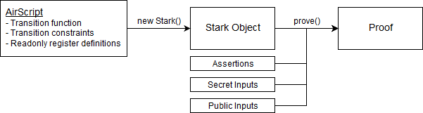
First, I want to briefly describe all the components that come into play to when generating/verifying STARK proofs (a more in-depth explanation is here and here). Here is a high level diagram of how proofs can be generated:

image

In the above diagram:

  • AirScript code defines transition function, transition constraints, and readonly registers. This code is then “compiled” into a Stark object.
  • Stark object is used to generate proofs. You can generate many proofs using the same Stark object by providing different assertions (same as boundary constraints), secret and/or public inputs.

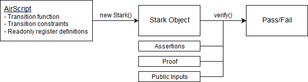
Verification of a proof works in a similar manner, except the verifier does not need to supply secret inputs to the verify() method:

image

Merkle Proof

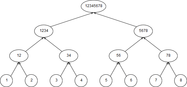
Let’s say we have a Merkle tree that looks like this (numbers in the circles are values of the nodes):

image

For illustrative purposes I’m assuming that hash(a,b) = ab. For example, hash(3,4) = 34 and hash(4,3) = 43.

A Merkle proof for leaf with index 2 (node with value 3) would be [3, 4, 12, 5678]. To verify this proof we need to do the following:

  1. Hash the first two elements of the proof: hash(3,4) = 34
  2. Hash the result with the next element of the proof: hash(12,34) = 1234
  3. Hash the result with the next element of the proof but now the result should be the first argument: hash(1234, 5678) = 12345678

Execution Trace

Now, let’s translate the above logic into an execution trace that we can later convert into a STARK proof.

First, let’s say we have a hash function that works like this:

  1. The function requires 4 registers to work and takes exactly 31 steps to complete.
  2. To hash 2 values with this function, we need to put the first value into register 1 and the second value into register 2 (the other 2 registers can be set to 0).
  3. After 31 steps, the result of hashing 2 values will be in register 1.

Our execution trace will have 8 mutable registers - 4 registers for computing hash(a,b) and the other 4 registers for computing hash(b,a). These registers are named r0 - r7. We also need a few readonly registers:

  • k0 - this register will control transition between invocations of the hash function.
  • p0 - this is public input register that will contain a binary representation of the index of the node for which the Merkle proof was generated. In our case, the index is 2 so the binary representation is 010.
  • s0 - this is a secret input register that will contain elements of the proof.

Now, since we need to invoke the hash function 3 times, and we need a step between each invocation to figure out which values to hash next, our execution trace will have exactly 96 steps (for the purposes of this example I’m not requiring the trace length to be a power of 2):

Step k0 p0 s0 r0 r1 r2 r3 r4 r5 r6 r7
0 1 0 12 3 4 0 0 4 3 0 0
1 0 12
31 0 0 12 34 43
32 1 1 5678 34 12 0 0 12 34 0 0
1 1 5678
63 0 1 5678 3412 1234
64 1 0 1234 5678 0 0 5687 1234 0 0
1 0
95 0 0 12345678 56781234

Here is what’s going on:

  1. [step 0]: we initialize registers r0 - r7 as follows:
    a. First element of the proof (3) is copied to registers r0 and r5.
    b. Second element of the proof (4) is copied to registers r1 and r4
    c. All other mutable registers are set to 0
  2. [step 31]: after 31 steps, the results of hash(3,4) and hash(4,3) are in registers r0 and r4 respectively. Now, based on the value in register p0 we decide which of the hashes advances to the next step. The logic is as follows: if p0=0, move the value of register r0 to registers r0 and r5 for the next step. Otherwise, move the value of register r4 to registers r0 and r5.
    a. In our case, at step 31 p0=0, so the value 34 moves into registers r0 and r5 for step 32.
  3. [also step 31]: At the same time as we populate registers r0 and r5 with data for the next step, we also populate registers r1 and r4 with data for the next step. In case of r1 and r4, these registers are populated with values of register s0 which holds the next Merkle proof element.
    a. In our case at step 31 value of s0=12, so 12 moves into registers r1 and r4 for step 32.
  4. After this, the cycle repeats until we get to step 95. At this step, the result of the proof should be in register r0.

In my prior posts I’ve shown an AirScript transition function that would generate such a trace. Here is a simplified version:

when ($k0) {
  // code of the hash function goes here
}
else {
  // this happens at steps 31 and 63 (technically at step 95 as well, but doesn't matter)

  // select the hash to move to the next step
  h: $p0 ? $r4 | $r0;

  // value h goes into registers r0 and r5
  // value from s0 goes into registers r1 and r4
  out: [h, $s0, 0, 0, $s0, h, 0, 0];
}

And here is how transition constraints for this would be written in AirScript:

when ($k0) {
  // code of the hash function constraints goes here
}
else {
  h: $p0 ? $r4 | $r0;
  
  S: [h, $s0, 0, 0, $s0, h, 0, 0];

  // vector N holds register values of the next step of computation
  N: [$n0, $n1, $n2, $n3, $n4, $n5, $n6, $n7];

  // this performs element-wise subtraction between vectors N and S
  out: N - S;
}

Readonly registers

A bit more info on how values for readonly registers (k0, p0, s0) are set:

As I described previously, k0 is just a repeating sequence of 31 ones followed by 1 zero. It works pretty much the same way as round constants work in your MiMC example. Within AirScript k0 is considered to be a static register are the values for this register are always the same.

Values for p0 are calculated using a degree n polynomial where n is the number of steps in the execution trace. The polynomial is computed by generating the sequence of desired values (e.g. for index 010 it would be 32 zeros, followed by 32 ones, followed by 32 zeros), and then interpolating them against lower-order roots of unity. Since the verifier needs to generate values for this register on their side as well, p0 register is considerably “heavier” as compared to k0 register. But for execution traces of less than 10K steps (or even 100K steps), the practical difference is negligible. Within AirScript, p0 is considered to be a public input register as its values need to be computed at the time of proof generation and verification and so must be known to both the prover and the verifier.

Values for s0 are computed in the same way as values for p0 but unlike p0 the source values are not shared with the verifier. Instead, values of s0 are included into the proof in the same way as values of mutable registers. From the verifier’s standpoint, s0 is almost like another mutable register, except the verifier does not know a transition relation for this register. The verifier is able to confirm that values of s0 form a degree n polynomial where n is the number of steps in the execution trace.

This is not really a problem given our transition function and constraints. Basically, what the verifier sees is that every 32 steps an unknown value is copied into registers r1 and r4, and then this value is used in hash function calculations that produce the desired output. Within AirScript, s0 is considered to be a secret input register as the verifier is not able to observe source values for this register.

Boundary constraints

The only boundary constraint that we need to check here is that at the end of the computation we get to the root of the Merkle tree. If everything worked out as expected, the root should be in registers r0 or r4 (depending on wither the index of the leaf node is even or odd).

1 Like

Thanks! This is really helpful.

Great! If you (or anyone else) see any issues or have any concerned about the methodology I outlined above - do let me know :slight_smile:

I did have one more question for you: in your MiMC example, you build a Merkle tree of P, D, and B evaluations (source) ; then you use the root of this tree to compute linear combinations of P, B, and D; and then you build another Merkle tree from these linear combinations (source).

My question is: for the first Merkle tree, do we really need to include values of P, D, and B? Could we get away with just using values of P to build it? Here is how I’m thinking about it:

The prover builds the first Merkle tree using values of P evaluations only (mTree). Then uses the root of mTree to compute linear combinations of P, D, and B, and then builds another tree from the resulting values (lTree). This last part is the same as in your example.

The verifier then does the following:

  1. Verifies that values of all spot check of P are indeed a part of mTree (this is done via Merkle proofs against mTree root - same as in your example).
  2. Uses these values to compute values of D and B for each spot check.
    a. D value can be computed as C(P(x)) / Z(x)
    b. B value can be computed as (P(x) - I(x)) / C(P(x))
  3. Computes linear combinations of P, D, and B using mTree root (same as in your example).
  4. Verifies that linear combinations for all spot checks are a part of the lTree (this is done via Merkle proofs against lTree root - same as in your eample).

Would this approach compromise security somehow?

Interesting! I think that might actually work…

If it does work, that would be really cool! I quickly implemented this simplification in this pull request and the results are:

  • About 3% - 4% proof size reduction for something as simple as MiMC.
  • About 20% proof size reduction for something slightly more complex (e.g. Merkle proof). For example, proof of a Merkle branch verification for a tree of depth 16 is now 109 KB (vs 136 KB before).

In general, the more complex the STARK (i.e. more transition and boundary constraints), the greater the impact. Though, I’d expect the impact to be smaller for proofs with long execution traces (there, proof size is dominated by FRI proofs).

109 KB… nice! If you crank up the code redundancy from 8x to 16x and do 2**20 proof of work on the Merkle root and then decrease the branch count based on that (the code redundancy should let you decrease by 25%, and the PoW by another ~20%) then it seems like we’re close to these STARKs fitting inside a block!

Adding proof of work to the Merkle roots is a very cool idea (and it’s pretty simple to do)! Here is how I’m thinking of implementing it:

  1. Compute a nonce such that hash(nonce | root) < threshold.
  2. Then, use this nonce as a seed to PRNG used to generate indexes for spot check.

The nonce would be included in the proof, and the threshold parameter could be configurable. Also, I’m guessing this technique could be applied to the main Merkle tree (mTree) and Merkle trees in the FRI proof - right?


As I was writing this, another potential optimization idea came to mind:

Right now, the proof includes spot-checks against several Merkle trees. Specifically: spot-checks against mTree (source), spot-checks against lTree (source), and spot checks against m and m2 trees in the FRI proof (source). It might be possible to roll spot-checks against lTree into the FRI proof at no extra cost. Here is how I’m thinking about it:

During the first pass of the FRI proof function, lTree and m are actually the same trees. This is because the values passed into prove_low_degree() function are just evaluations of the linear combination (source).

We might be able to use spot-checks against m tree from the first element of FRI proof instead of spot-checks against lTree to validate the correctness of linear combination. It would work like this:

  1. Build mTree in the same way as it is done now.
  2. Compute linear combination of evaluations in the same way as is done now - but don’t put them into a separate Merkle tree.
  3. Run FRI proof. The first component of the FRI proof will contain spot-checks against m tree which is a tree of all linear combinations.
  4. Use the same indexes as were used to spot-check m tree in the first component of the FRI proof to spot-check the mTree.

The problem is that this undermines security somewhat. By manipulating composition of FRI proof trees, the attacker could theoretically try to hit the “right” indexes in the mTree and fake the proof. But I wonder if adding proof of work requirement to building the trees is enough to offset this reduction in security.

If it does work, it would reduce the proof size by about 10%.