This work was done by the Codex team, and we would like to thank @dankrad, @matt, @Nashatyrev, @oascigil, @fradamt, @pop and @srene for their feedback and contributions to this work.
TL;DR
This work attempts to answer most of the questions raised in the original PeerDAS post regarding sampling, data custody, network requirements, and honest byzantine ratios.
- Under normal conditions and relatively low networking assumptions, the network can quickly perform sampling while guaranteeing high decentralization.
- The network is robust enough to absorb large correlated failures in which more than a third of nodes do not contribute to the sampling process.
- Large coordinated attacks of a dishonest majority (90%) are still a challenge that need to be addressed with other techniques.
Introduction
The Ethereum network has been running with EIP4844 since the DenCun (Deneb-Cancun) fork on March 13th, 2024. In the current conditions, nodes have to download a maximum of 6 blobs, each 128KB size. When full DAS comes to life, we expect much more data to be produced at every slot. The current planned structure is a 2D matrix of 512 rows by 512 columns (after erasure coding), in which each cell is 560 bytes in size (including KZG proofs). That makes each row/column have a size of 280 KB for a total matrix size of 140MB. Of course, these numbers can change, but we will use this estimate for this analysis.
Assumptions
Full DAS includes two main components: data-sharding and sampling. Data-sharding refers to the fact that the nodes in the network are not required to download the entire block/blobs but only a part of it. Sampling is the process by which nodes verify whether a block is available without downloading the whole block.
Custody
Before sharding the data into rows and columns, dispersing it over the P2P network, and sampling it, we must explain how nodes know what data they are responsible for. Nodes use their nodeID and custody_size to derive, deterministically, which rows and columns they need to have custody of. The custody_size is the number of rows and columns a node wants custody of, and it is transmitted inside the Ethereum node records (ENRs) during the discovery process. More on this later. For instance, a node that wants to have custody of 16 rows and columns will generate a SHA-256 hash of its own nodeID, then cut this 256-bit hash into 25 segments of 10-bit (discarding the last 6 bits), and those 10-bit numbers (from 0 to 1024) will be the list of rows and columns the node must have custody of. In this case, 25 is not enough because we need 32 (16 rows and 16 columns), then we simply increment the nodeID by one, SHA-256(nodeID+1), to get another 25 row/column IDs. This process can be repeated as many times as necessary. If any ID is repeated, we simply disregard it and take the next one until we reach our quota. This process needs to be done only once when the node is initialized. Please note that any node can do the same computation for all its peers because it has the nodeID and custody_size of all of them. Therefore, all nodes in the network know which data is under the custody of all their respective peers. This algorithm is just an example of implementing deterministic custody; many other options exist.
Data Dispersal
For data dispersal, we assume that nodes download the part of the data they need to have custody of, from the block builder. They download the data using GossipSub channels in the same way they are used today for attestations, blocks, aggregations, etc. We assume a total of 1024 GossipSub channels (512 rows and 512 columns), and the nodes in the network subscribe to the channels required to satisfy their custody needs. This strategy relies on the premise that GossipSub should scale efficiently to over a thousand channels, which has never been tested on a production network like Ethereum Mainnet. Nonetheless, it is not overly optimistic to assume this can be the case in the near future. We also assume that nodes do not change their custody set frequently, only when they restart the node with a new nodeID, so they remain subscribed to these GossipSub channels for extended periods (e.g., months). Also, we assume that only half of the row/column is sent over the network, and the other half is reconstructed on the fly using Reed-Solomon encoding. This means that a node that wants to download the entire block (140 MB) only needs to download 256 rows, and only half of the row is received (32 MB). The node can then extend the received 256 half rows horizontally and then generate the missing 256 rows by extending the data vertically. In other words, if the node has custody of 256 or more rows/columns, it can regenerate everything from only 32 MB of data.
Sampling
For sampling, we assume that nodes can query each other through a lightweight communication channel (e.g., new discovery protocol, lightweight libp2p, etc) in which one can establish ephemeral connections that only last for a couple of seconds. Such a protocol does not exist today, but it is not unrealistic to believe we can implement this rather quickly. Most of the networking components already exist today. Given that the custody set is computed deterministically from the nodeID, any node in the network can know what rows and columns are in the custody set of its peers.
In addition, we also assume a P2P network similar to the current Ethereum network, which has about ten thousand nodes, and we also assume that all clients can handle a couple hundred peer connections in parallel without overhead issues, which seems realistic given that consensus layer (CL) clients today can easily maintain connections with about a hundred peers.
Objective
In this study, we analyze how difficult it would be to sample a block in full DAS using the network assumptions given above. Therefore, we model a P2P network in which every node has a certain number of peers P, and a custody set of C rows and columns of the 2D matrix. Then, we investigate how these two parameters impact the speed at which sampling is done.
In particular, we look at the number of hops necessary for sampling. For instance, when a node wants to sample a given cell, it looks around its peers to find who has custody of the row or column of that cell and then sends the query. If none of its peers has that cell in custody, it sends the query to a random peer. The peer receiving the query cannot send the cell, therefore, it will answer with a list of its peers that have it in their custody set. The original node can now send the query to any of those peers, resulting in a two-hop sampling process. The same procedure can be repeated as deep as needed (H hops) until finding a node with the cell in its custody set.
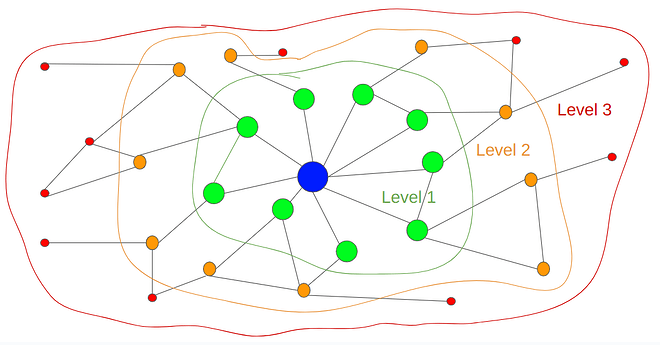
We give this concept the name of sampling horizon. We call the level 1 horizon, the set of cells that a node can “see” by querying his direct (one-hop) peers. In the figure above, the level 1 horizon of the blue node is represented by the cells of the 2D matrix that are in the custody set of the nodes in green. The level 2 horizon is the set of cells a node can “see/sample” from its direct peers and their direct peers (up to two hops), i.e., the cells in the custody of the green and orange nodes in the figure.
The concept of sampling horizon, as defined in this work, is closely related to the degrees of separation from network theory. For instance, some studies predict that all humans are connected by six degrees of separation. However, it is essential to distinguish between the two concepts: degrees of separation is the metric that defines the distance between two nodes in the network, while the sampling horizon, as described here, is the set of cells a node can see within x degrees of separation. This can also be described as the set union of custody of nodes within x degrees of separation.
Given all this, we try to answer the question: how much cell coverage do we get on the level 1 horizon, level 2 horizon, and so on for a specific network configuration? This would depend mainly on two parameters: the number of peers P of the nodes and their custody size C. Let’s assign some values to them.
Methodology
In this section, we explain how we assign values to the custody size and the number of peers.
Flat Custody
Custody refers to the responsibility of nodes for storing specific data partitions (rows and columns) within the decentralized network. Flat custody is an approach where each node is assigned an equal number of rows and columns to its custody set, regardless of how many validators the node has. For example, we could set the custody to be two rows and two columns (C=2) for all the nodes in the network and then evaluate how much cell coverage we get at horizon level 1, level 2, and so on.
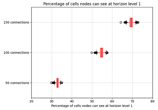
The figure above shows the percentage of cells a node can see at horizon level 1, assuming C=2 and for different values for P (50, 100, and 150). For every node in the entire P2P network, we compute the percentage of cells from the entire 2D matrix that it can see in its level 1 horizon. The figure shows the median, the 1st and 3rd quartiles, the whiskers, and the outliers. As we can see, the more peers a node has, the more extensive the level 1 horizon coverage becomes, up to 70% for P=150 peers. Block sizes impact data propagation, so analyzing the amount of data nodes need to download is essential. In this scenario, all nodes need to store, and therefore download, 22512*560 = 1MB of data at every slot, which is not far from the ~900KB a node has to download today under EIP-4844 for a block with six full blobs.
However, flat custody is not a fair data partitioning strategy because the network has many different types of nodes. Running a small node without validators at home is not the same than running a beefy node with hundreds of validators in the cloud. Those are two very different conditions because of the hardware they have, the network bandwidth they use, the amount of value they store, and the revenue they produce. Therefore, we propose another approach that considers the number of validators running in the node and the expected resources involved proportionally.
Validator Proportional Custody
Under the validator-proportional (VP) custody model, the custody allocation is based on the number of validators a node has. This ensures that nodes with more validators take on more responsibility, distributing the network load more efficiently according to node capacity.
Custody Model
In VP custody, we define the total custody of a node with the following equation:
total_custody = min_custody + floor(val_per_node × val_custody)
where
- Minimum Custody (min_custody) is the minimum number of rows and columns every node should custody. This ensures that every node, regardless of its validators, takes on a base level of responsibility for data.
- Validators Per Node (val_per_node) refers to the number of validators a node has. It is a property of the node. Different nodes have different values of val_per_node.
- Custody Per Validator (val_custody) represents the number of rows and columns a validator in a node is assigned. It is a property of the network. All nodes in the network will have the same val_custody value. Note that this parameter can take a fractional value such as 0.5, and the nodes will add one row/column for every two validators they host.
Model Parametrization
Now that we have a custody model, we need to give values to the parameters of that model.
Validators per node
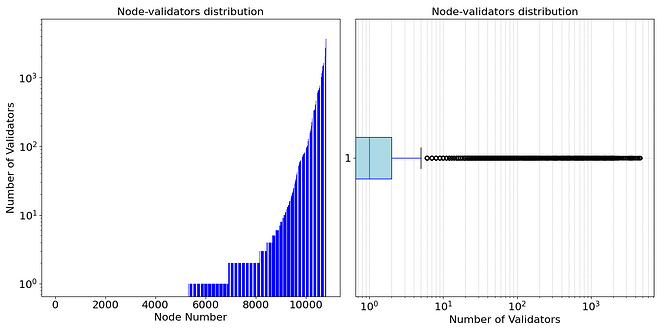
To model a network using validator-proportional custody, we need to know the distribution of validators across the network. The number of nodes in the Ethereum network today is well-known thanks to several crawlers that have been developed in the past. However, the number of validators per node is a more tricky issue. In our previous research work, we used the past attestation topic subscription plus other extra data to infer the number of validators hosted in the nodes. According to that study, about 10% of the nodes had 64 or more validators, while 80% had none or just a few validators, and the heaviest node in the network hosts about 3000 validators. This work uses the same distribution of validators per node, as shown in the figure below. Please note that even if we have the list of the nodes in the network and estimate the distribution of the number of validators per node, we still cannot determine the exact number of validators each node has. Thus, in our simulations, we assign to each node, a random number of validators from the values observed in this given distribution. In this way, we can recreate the same distribution presented here.
Custody per validator
To assign a value to the val_custody parameter, we can start by asking when a node should download the entire block. Let’s pick an arbitrary number, for example, 1 row/column per validator. From the moment the node downloads 256 rows, it can automatically regenerate the other half of the data using Reed-Solomon encoding, ending with the custody of the entire block, becoming a data availability (DA) provider. It is essential to note that in this scenario, the node will not need to download both rows and columns; either rows or columns is enough because it will have the entirety of the data after erasure coding. Then, let’s proceed with an economical analysis of a node with 256 validators. Such a node is securing ETH 8192, equivalent to over USD $20M+ as of today’s price. Therefore, it seems reasonable to assume that a node with that much capital has the economic resources and incentives to run that node in the very best hardware and network conditions. Such a node should be able to download and reconstruct every block quickly. Thus, we can set val_custody=1 so that a node with 256 validators will have custody of the entire block. This parameter can change if we want to increase/reduce the custody size of nodes and the number of DA providers in the network, as we will see in a later section.
Minimum custody
We use a different approach to set a value to the min_custody parameter. In this case, the objective is to minimize the amount of data a small home node without validators needs to download and store. As we saw in the Flat Custody section, a node with a custody size of 2 rows and columns must download about 1MB of data per slot, which is reasonably close to the case of a block with six blobs today. Thus, for the remainder of this study, we set min_custody=2.
Number of Peers
In the preliminary results of the flat custody, we tested a different number of peers, from 50 to 150, which are realistic values today, as we have seen in previous studies. However, one aspect of that simulation that could be more realistic is making the number of peers not the exact same value for all nodes. While most clients stay within the same range, different CL clients have different default values for the number of peers. Thus, we adapted the code of our simulator to give a range for the number of peers instead of a value. All nodes randomly choose a number of peers within the range given as a parameter. For example, we could study what happens when the number of peers ranges between 50 and 100, 100 to 150, and 150 to 200. We could further explore what happens when we increase these ranges, as we will see later.
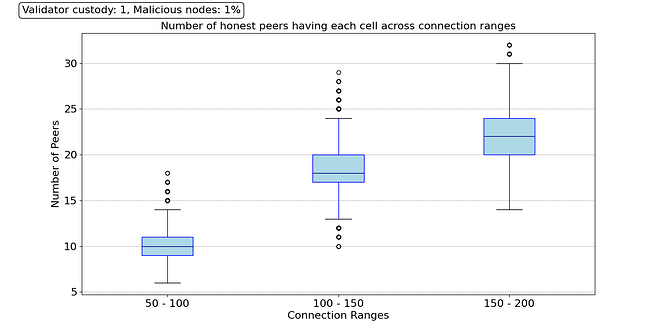
Thus, we study the sampling performance using these three ranges for the number of peers P and the same parameters for custody C as in the previous section (i.e., min_custody=2, val_custody=1). For example, we can ask one question: for one particular cell, how many direct peers (level 1) have custody of this cell? Then, we can repeat the same question for another cell, and another, and so on, until we have the answer for all the 262,144 cells in the block. Then, we can plot that distribution for the three different P ranges. The results are presented in the figure below.
We can see that on average, even for a connectivity range of 50 to 100 peers, most cells are under the custody of around ten directly connected peers (level 1). As we increase the number of peer connections, the level 1 horizon increases, thus increasing the reliability of the distributed network. For a range of 150 to 200 peers, the cells of the block can be found in about 33 direct peers on average, and all cells are under the custody set of at least 20 direct peers.
Evaluation
In this section, we perform several simulations to evaluate the sampling performance under multiple scenarios. We are interested in two key metrics:
- The level 1 horizon: This allows us to get an idea of the percentage of queries that can be answered quickly (1 hop). It also shows the network’s reliability level because it indirectly expresses the data redundancy in the network. For this metric, the higher, the better.
- The amount of data downloaded by each node: This shows the network requirements that the different types of nodes should have to run a node. This is directly related to the level of decentralization of the network. For this metric, the lower, the better.
Happy Case
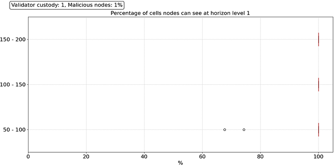
The first scenario we look at is the “happy” case in which 99% of the nodes behave correctly and have no performance issues of any type, neither network data loss nor hardware failures. Using the proportional custody model and parameters defined above, the cell coverage of the level 1 horizon improves dramatically over the flat custody model presented previously, as shown in the figure below.
All nodes can access all cells within one hop, and this is for all three ranges of the number of peers, except for a couple of outliers in the range of 50-100 peers. This is because, under the proportional custody model, nodes generally have larger custody sets and also due to the presence of DA providers —nodes with 256 or more validators— within their level 1 horizon.
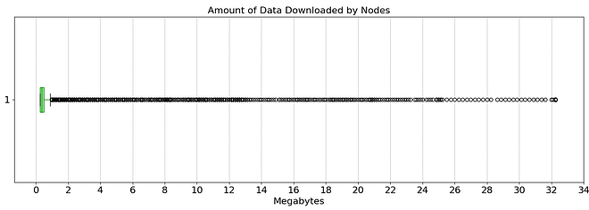
Regarding the amount of data that needs to be downloaded, we can see in the figure above that most nodes download less than 1 MB of data per slot. Only a few outliers, mostly DA providers, download over 2MBs of data up to the totality of the block (~32MBs). These results show that it is possible to perform fast sampling under ideal conditions while keeping the download needs for most nodes low. This is an ideal outcome because it guarantees high security and high decentralization. Now, let’s analyze what happens under more catastrophic scenarios.
Correlated Failures
In this section, we demonstrate what happens when there is a correlated failure in which a given feature is correlated within a large set of nodes, and this feature is the root cause of the failure. Thanks to our open-source network crawler at MigaLabs, we have detailed information about all the nodes in the consensus layer network, including their ISPs, geographical locations, and the CL clients they are using. This data enables us to selectively simulate the shutdown of specific groups of nodes based on those criteria.
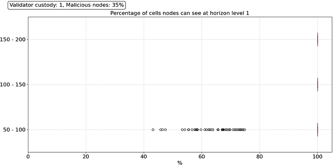
We look at three scenarios regarding CL client diversity, geographical distribution, and type of hosting. For instance, if a majority CL client (i.e., Lighthouse) deploys a new release with a bug that renders the nodes incapable of syncing, we could see over 35% of the nodes go down in a very short time. The same could happen if the country with the highest node concentration (i.e., USA) suddenly bans crypto because of a new presidential candidate been elected, for example. A similar scenario could occur if the three larger cloud providers used in the Ethereum network (i.e., AWS, Hetzner, and OVH) decide to ban all crypto-related activity simultaneously. Thus, we simulate what happens when 35% of the nodes suffer from a correlated failure and stop providing samples and forwarding requests of any type.
Before analysing the reliability of the system, let us do a network bandwidth analysis. The amount of data that needs to be downloaded is not affected by the number of nodes failing. Hence, the bandwidth requirements stay the same. Downloading the data can take longer because many nodes will not forward anything on the Gossipsub channels. Therefore, more requests should be sent which has negligible bandwidth, but it has delay implications. This work focuses only on custody and sampling aspects; data dissemination is out of the scope of this article. For dispersal simulations, please refer to our previous paper.
Regarding the robustness of the sampling process, we can see in the results above that the network is highly reliable, even under such a catastrophic failure, and 99.9% of the nodes can perform fast sampling (1 hop) without any issues. The only outliers are some nodes in the 50 to 100 peers range that only see between 40% and 75% of the cells within their level 1 horizon. They will need to reach their level 2 horizon (2 hops) to satisfy their sampling needs, which means their sampling performance will be lower, but it does not mean they will necessarily fail the sampling process.
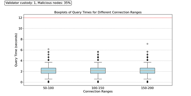
To understand how much those outliers can perturb the network, we compute how much time 75 sampling queries take for all the nodes in the network. To do this, we assign a sampling time for querying a level 1 node st1 and a level 2 node st2. We also set a timeout for when a node queries a malicious peer, and this peer does not answer. In this case, the node must launch a second query to another peer. Most nodes in the Ethereum network show an RTT of about 100ms. Therefore, we give our time parameters the following values: st1=100~200ms, st2=200~300ms, and to=500ms. Please note that all sampling queries are launched in parallel; the only queries executed sequentially are those launched after a timeout.
In the results shown above, we can see that, even under this catastrophic failure, the large majority of nodes can perform their sampling duties within 4 seconds. Those taking more time are nodes that contacted multiple malicious nodes consecutively. These encouraging results indicate the possibility of reaching high security, even under highly correlated failures, without compromising decentralization.
Byzantine Attacks
Now, we want to take things to the extreme and simulate a coordinated attack in which a large majority of the nodes (90%) decide to behave maliciously by withholding the data and not answering/forwarding sampling requests. We simulated cases in which 60%, 70%, 80%, and 90% of the nodes in the network behave maliciously, but for brevity in this writeup, we only show results for the worst case: 90% of nodes are malicious, regardless of their number of validators. This means that even DA providers can be malicious and withhold data.
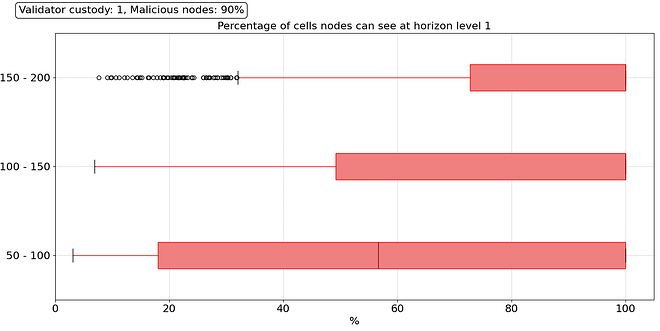
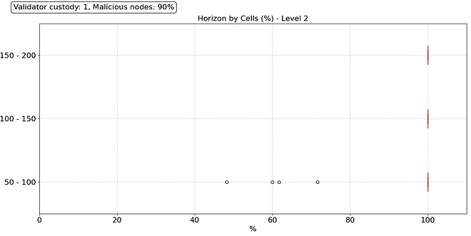
In this scenario, we see a dramatic difference in the level 1 horizon. The distribution is catastrophic for all peer ranges. A massive proportion of the nodes have only a partial view of the block on level 1. Looking at level 2, things improve, primarily due to the presence of honest DA providers in their level 2. However, having an honest DA provider at reach does not guarantee good sampling performance because, with 90% of malicious nodes, it is difficult to reach an honest one by pure random trial. In this attack, we assume that even malicious nodes behave correctly for some time until they decide to launch the attack. Under those circumstances, finding an honest node becomes exceptionally challenging, even using reputation mechanisms.
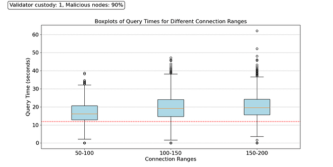
Under these conditions, nodes will contact malicious nodes many times in a row, leading to long sampling times. We calculate the sampling time for all nodes for all three different peer ranges, and plot the distributions in the figure above. We see that the majority of the nodes take over 15 seconds to finish their sampling. However, in the Ethereum protocol, there are time constraints, and nodes cannot wait forever to decide whether a block is available or not. For this experiment, we set a hard final timeout fto, which represents the break time when, if the 75 sampling queries have not finished successfully, the nodes decide the block is not available. For this example, we set fto=12s, see the red dotted line in the figure.
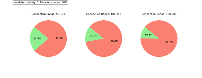
Under this scenario, only a few nodes manage to finish their sampling queries in time. An unexpected result of this experiment is that as we increase the number of peers, the distribution of the sampling duration widens up, and fewer nodes manage to finish sampling in time, as shown in the figure below. When we have many direct peers, we have a large pool of malicious nodes to whom we might inadvertently send a sampling query. This means that under such a large coordinated attack, having a large number of known peers does not help because the node is unaware of which ones are malicious and which ones are not. In these conditions, other techniques are necessary.
Mitigating Malicious Majority Attacks
Increased Replication
One way to try to mitigate these types of attacks is by increasing the amount of data replication in the system. This can be done by increasing the validator custody so that nodes with validators have custody of more rows and columns, and this also lowers the bar to become a DA provider, which in turn increases the number of DA providers in the network. For instance, if we set val_custody=4, any node with 64 validators should become a DA provider, and there would be much more replication in the network. However, this is not enough to mitigate this attack, and our simulations show that only between 15% and 22% of the honest nodes see the block as available. In addition, this also increases the bandwidth requirements for all nodes, which is an undesirable effect of this strategy.
Lossy Sampling
Lossy sampling is another strategy that allows nodes to tolerate one or several failed queries in the sampling process. This is particularly useful when one sample or a few samples are missing. However, lossy sampling is of little help for this massive coordinated attack. Under such conditions, most nodes do not even finish half of their requests; therefore, allowing a few failed queries will not absorb the Byzantine’s faults in any meaningful way.
Discussion
In this work, we have studied the sampling process under full DAS, considering a set of assumptions, mostly related to the network layer and a few others, such as the validator distribution. We have demonstrated that under fair networking conditions, DAS sampling is not only achievable but it can be performed rather fast. We have presented a number of parameters with which researchers can play to move the needle between decentralization and reliability. The study also shows how the network can absorb large correlated failures and still perform sampling reliably.
However, this work has several limitations:
- During the entire work, we assumed that nodes select peers randomly. In reality, nodes can tune their peers to improve their level 1 and level 2 horizons, which should lead to much more robust networking conditions. In some sense, the results presented in this work can be viewed as the baseline from which many improvements can be achieved by enhancing the peering algorithm.
- We assume that when a node does not have a cell in its horizon level 1, then it contacts a node randomly to try to reach a potential level 2 node. There are other strategies that can be considered and that we have not considered in this work. For example, topicID routing could improve performance in this context.
- The whole study was performed assuming that the nodes only know a small set of nodes and they sample only from that set. However, peer discovery algorithms can run in parallel, and nodes can store a rather large number of peers in their database. It is not impossible to contact thousands of peers while syncing and start the whole sampling process with a huge level 1 horizon.
- This work assumes a rather static view in which the horizon of the nodes does not evolve. However, this is not realistic. As nodes discover other peers, their horizon is constantly evolving and with it the sampling performance.
- We have shown results for only a network of 10K nodes and a specific validator distribution. However, both the size of the network and the validator distribution can change in the coming years. Thus, it is necessary to perform experiments under those conditions.
Conclusions
This work demonstrates that under certain realistic networking assumptions, it is possible to perform fast sampling at scale. The study also shows that with the presented strategies, the network can even absorb large correlated failures. However, malicious majority attacks remain a challenge and should be further studied.
Acknowledgments
This research was done with the support of the Ethereum Foundation under grant FY24-1533.
