By @cskiraly, @leobago, and @dryajov from the Codex team.
The aim of this post is to share some of our DAS related findings with the community. These have been shared with some of you already last year, and for reference we link the original documents. Here below we hope to provide a more digestible summary.
TL;DR
- An important parameter of DAS is the sample size, i.e. the number of segments (or columns) a node downloads and verifies. It is sometimes better to allow a few missing segments and have a slightly larger sample size than to have a smaller sample size but try to retrieve all segments of the sample at all costs. We call this technique LossyDAS.
- It is possible to gradually increase the sample size, extending the sample if the test fails (or does not conclude in, e.g. a given time). We call this strategy IncrementalDAS.
- When selecting what to sample on a 2D Reed-Solomon encoded grid, the usual assumption is to use a uniform random choice. We show that choosing row and column distinct samples, which we call DiDAS (“distinct” or “diagonal” DAS), provides probabilistically better results. It is trivial to implement, while it doesn’t seem to have any disadvantages.
Intro
Sharding and DAS have been in the works for some time now. While the initial paper and the Danksharding proposal focused on a 2D Reed-Solomon (RS) encoding, some recent posts are proposing a transitional one-dimensional encoding. In this post, we focus on some aspects of sampling and its probabilistic guarantees, and we propose three improvements to the system. The techniques described below have been developed for the case of the original 2D RS encoding, but to some extent apply also to the transitional proposals.
First, we introduce lossy sampling for data availability (LossyDAS), which provides the same probabilistic guarantees as random uniform sampling, adding error tolerance in exchange for slightly larger sample sizes.
Second, we discuss IncrementalDAS, which provides the basis for developing a dynamic sampling strategy with increasing sample sizes.
Finally, we introduce diagonal sampling for data availability (DiDAS), a method that improves sampling performance over this specific 2D erasure code, providing better performance than uniform random sampling for worst-case “adversarial” erasure patterns.
Sampling over the DAS encoding
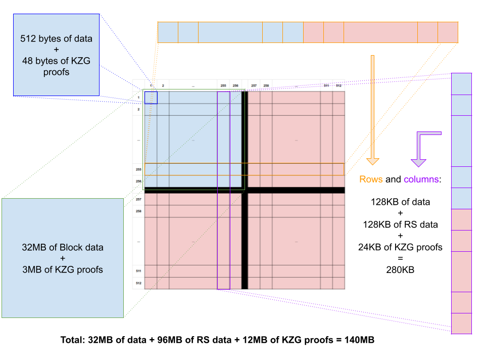
Figure 1: Data Availability encoding structure
Figure 1 shows the 2D data availability encoding as proposed in Danksharding, using a square structure, using the same RS code with K=256 and N=512 in both dimensions. This means that any row or column can be fully recovered if at least K=256 segments of it are available.
In the baseline sampling process, a sampling node selects S segments uniformly random without replacement, and tries to download these from the network. If all S can be retrieved, it assumes the block is available. If at least one of these fails, it assumes the block is not available.
Sample Size and Erasure Patterns
An important parameter of DAS is the sample size S, i.e. the number of segments a node downloads and verifies. When evaluating how many samples are needed, it is important to note that, contrary to a simple RS code, a multi-dimensional code is non-MDS (maximum distance separable). With an MDS code, repairability only depends on the number of segments lost, but with a non-MDS code, it depends on the actual erasure pattern as well. This means that, with some probability, non-trivial erasure patterns will happen. Even more importantly, this potentially allows malicious actors to inject crafted (adversarial) erasure patterns in the system. Therefore, when analyzing the sampling as a test, we should differentiate between the cases of
- random erasures,
- adversarial (e.g. worst-case) erasure patterns.
Random Erasures
Random erasures are a plausible model when thinking of network and storage induced errors. The simplest model of random erasures is the case of uniform random erasures, which maps relatively well to the service provided by a DHT, as in the original proposal, when assuming honest actors. However, given the nature of the system, our main optimization target is not this, but worst-case or adversarial erasures.
Worst-case Erasures
When thinking of malicious actors, it is important to analyze worst-case scenarios. While the code is not an MDS code, we can describe what a worst-case (or minimal size) erasure pattern is. If we select any N-K+1 rows and N-K+1 columns, and remove all segments in the intersections of these selected rows and columns (i.e. 257 * 257 segments out of the 512 * 512 segments), we prevent any recovery from taking place. There are only full rows and unrecoverable rows, and similarly, there are only full and unrecoverable columns. No row or column can be recovered therefore, the data is lost.
It is easy to see that the above is the “worst-case”. First, observe that worst-case here means the least number of missing segments. In our context, this also means the minimum number of nodes/validators a malicious actor should control in order to perpetrate the attack. In the worst-case, there should be no possibility of repairing rows or columns. Assume there is a worst-case pattern that has less missing segments than (N-K+1) * (N-K+1). In that case, there would be at least one column or row that has less than N-K+1 missing segments. That column/row is repairable, which contradicts our assumption. ![]()
Note: The above proof assumes an interactive row/columns based repair process. Multi-dimensional RS codes can also be repaired using multivariate interpolation, as discussed here. The proof described in their paper also applies to our case, confirming these patterns as worst-case minimal size patterns.
Trivially, any erasure pattern that contains a worst-case erasure pattern, is also unrecoverable.
Setting the Sample Size
When setting the sample size, what we are interested in is to limit the probability of a not-available block passing the test, in other words the false positive (FP) rate, independent of the erasure pattern. Clearly, with uniform random sampling, assuming an erasure pattern that makes the block unrecoverable, the larger the pattern, the easier it is to detect. Therefore, it is enough to study the case of the smallest such patterns, i.e. the worst-case erasure pattern. This probability can be approximated by a binomial distribution or - even better - calculated exactly using a hypergeometric distribution with
- population size: N*N
- number of failure states in the population: (K+1)*(K+1)
- Number of segments: S
- Number of failures allowed: 0
This probability obviously depends on S, the sample size. In fact, our real question is:
How many segments do we need to reach a given level of assurance?
As shown on Fig. 2, if we have a 2D RS coding, K=256, N=512, and want this probability to be below 1e-9, we need S=73 segments. The figure also shows the theoretical cases of using a 1D RS code with the same number of segments and the same expansion factor, and the case of a 2D RS code with a smaller expansion factor.
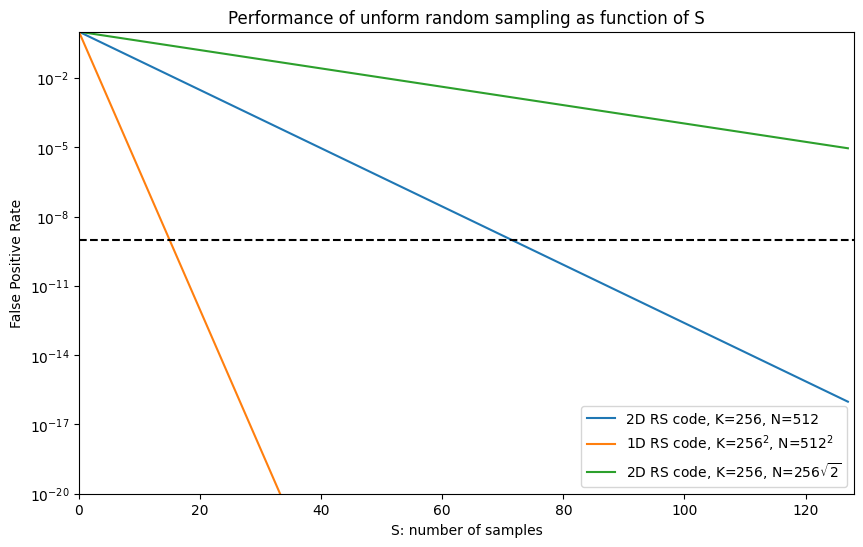
Figure 2: Performance of uniform random sampling over the DAS data structure, with different RS encodings, as a function of the sample size S
What about False Negatives?
As with all statistical tests, there are both cases of FP (false positives: the test passes even if the block is not available), and FN (false negative: the sampling fails even if the block is available). The ratio of false negative tests can be quantified using the survival function of the hypergeometric distribution as follows:
Where M is the size of the erasure pattern.
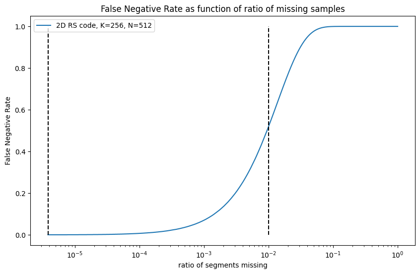
Figure 3: False Negative Rate as a function of missing samples
As an example, if there is only 1 segment missing out of the 512*512 segments, the probability of an FN test result is 0.03%. If instead 1% of the segments (2621 segments) are missing, the probability of an FN test is 51.9%.
So, how can this system work when there can be a large number of FN tests due to the unavailability of a few segments? More specifically, there are at least two issues here leading to FN cases:
- in a distributed setting with a large number of nodes, there are always transient errors, such as nodes being down, unreachable, or suffering network errors. Requiring all segments to be received means we should use reliable transport mechanisms (e.g. TCP connections, or other means of retransmission in case of failures) and even then, we need nodes to have relatively high availability and good network connectivity. Or, we need protocols that store data redundantly and retrieve it using multiple parallel lookups, like a typical DHT, and we still potentially need large redundancy and many retrievals.
- As we have seen, requiring all segments to be received also means that we might have a large amount of false negatives in our test if not all segments are actually available. In other words, the test easily fails when the data has some losses in the distributed structure, but it is actually reconstructable as a whole. While we could aim to avoid some losses by replication, retry, and repair, this might be very costly if not impossible due to the previous point.
To understand what can be done, let’s carefully analyze our basic premise until this point, focusing on a few key parts:
“When a node cannot retrieve all S of the selected segments, it cannot accept the block.”
- “cannot retrieve”: what “cannot retrieve” actually means in this context is something that needs more attention. It means we tried, and re-tried, and it was not retrievable. How long and with what dynamics should a node try to retrieve a segment? Should it also try to retrieve it by reconstruction using the erasure code? We argue that these network-level reliability techniques can be costly, and there is a trade-off between making the network more reliable and selecting the correct sampling process.
- “all”: do we really need to retrieve all segments? Wouldn’t it make sense to ask for more segments and allow some losses?
- “S”: Can we dynamically change S, looking for more samples if our first attempt fails?
To answer what “cannot retrieve” means, we should delve into the details of the networking protocols. We leave this for a subsequent post. Here in what follows, we discuss the two other possibilities. LossyDAS addresses the question of whether “all” samples are needed, while IncrementalDAS focuses on making “S” dynamic. DiDAS, instead, focuses on achieving the same probabilistic guarantees with a smaller “S”,
LossyDAS: accept partial sampling
Do we really need all segments of the sample? What happens if we test more segments, and allow for some losses? It turns out that we can define the test with these assumptions.
In LossyDAS, just as in the original test, we set the target FP probability (i.e., cases when the test passes, we think the data has been released, but it is actually in a non-repairable state). We look for the minimal value of S (the sample size) as a function of
- P_{FP}: the target FP probability threshold, and
- M: the number of missing segments we allow out of the S segments queried
In the calculation we use the percentage point function (PPF), which is the inverse of the CDF.
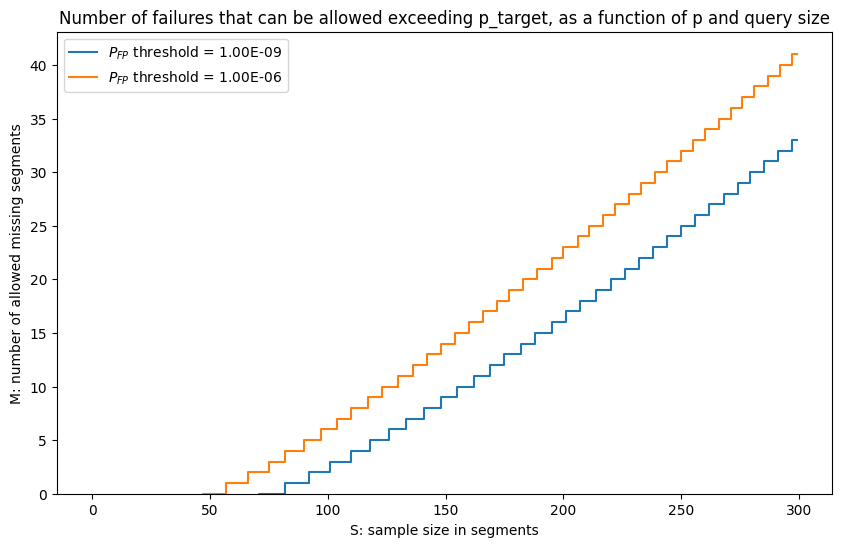
Figure 4: Number of failures that can be allowed is LossyDAS, respecting a given FP threshold
As we can see in Fig.4, we can sample slightly more and allow for losses while keeping the same FP threshold. For example, with a target FP of 1e-9, we can choose a sample size of 84 and allow 1 missing segment. Or we can go for 103 segments and allow up to 3 losses. In general, instead of sampling with n=73, approximately every 10 more segments allows us to tolerate one more missing segment.
In practice, this means that nodes can try to download slightly more segments, already factoring in potential networking issues or other transient errors.
IncrementalDAS: dynamically increase the sample size
What happens when too many segments are actually missing? Should we wait for these to be repaired, repair them on our own, or can we do something else? One might try to argue that the test should fail until all tested segments are repaired, otherwise the block is not available, but our whole system of probabilistic guarantees is built on the principle that repairability (and not repair) is to be assured. Moreover, waiting for it to be repaired might be too long, while repairing on our own might be too costly. The question that naturally arises is whether we can re-test somehow with a different sample.
First of all, we should clarify that simply doing another test on another random sample with the same S is a bad idea. That would be the “toss a coin until you like the result” approach, which is clearly wrong. It breaks our assumptions on the FP threshold set previously. If we make another test, that should be based on the conditional probabilities of what we already know. This is what IncrementalDAS aims for.
In IncrementalDAS, our node selects a first target loss size L1, and the corresponding sample size S(L1) according to LossyDAS. It requests these segments, allowing for L1 losses. If it receives at least S(L1) - L1 segments, the test passes. Otherwise, it extends the sample, using some L2>L1, to size S(L2). By extending the sample, we mean that it selects the new sample such that it includes the old sample, it simply picks S(L2)-S(L1) new random segments. It is easy to see that we can do this, since we could have started with the larger sample right at the beginning, and that would have been fine from the point of view of probabilistic guarantees. The fact that we do the sampling in two steps does not change this. Clearly, the process can go on, extending the sample more and more. L2 (and further extensions) can be decided based on the actual number of losses observed in the previous step. Different strategies are possible, also based on all the other recovery mechanisms used, which we will not detail here.
DiDAS: steering away from uniform random sampling
Until this point, it was our assumption that uniform random sampling is used over the erasure coded block structure. However, the code is non-MDS, and thus some segment combinations seem to be more important than others.
In the base version of the test, we select segments uniformly at random without replacement over the whole square. Some of these might fall on the same row or column, which reduces the efficiency of the test. If, instead of the base version, we make sure to test with segments that are on distinct rows and distinct columns, we increase our chances of catching these worst-case erasures. We call this sampling distinct (or diagonal) sampling for data availability (DiDAS).
Note: What we define here is a 2D variant of sampling without replacement. The diagonal is clearly a row and column distinct selection of segments, but of course there are many other possible selections. From the theoretical point of view, the whole erasure code structure is invariant to row and column permutations in the case of worst-case erasure patterns. Thus, when studying parameters, we can assume a sample in the diagonal and permutations of the erasure pattern.
How much we improve with DiDAS
With the new sampling method, the probability of catching a worst-case erasure from S segments can be expressed as a combination of two hypergeometric distributions. See our original working document (Jupyter Notebook) for the exact formulation. Fig. 5 shows the difference between the two sampling methods in the case of a worst-case erasure pattern.
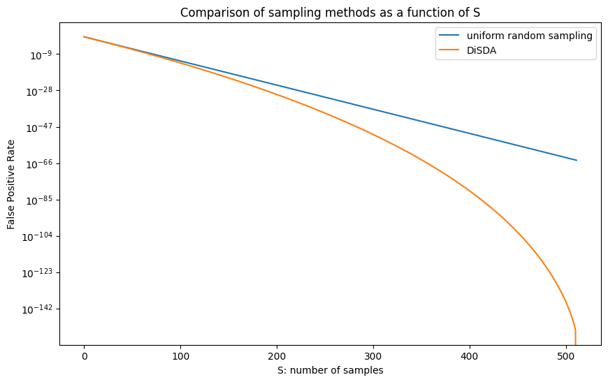
Figure 5: Comparison of uniform random sampling with DiDAS, with N=256, K=512, and a worst-case erasure pattern
Intuitively, for small S the difference is negligible: even if we don’t enforce distinct rows and columns, the segments sampled will most probably be on distinct rows and columns. S=73 is still relatively small in this sense.
For larger S, the difference becomes significant on a logarithmic scale, as in Fig. 5. However, we are speaking of very small probabilities, and we admit that it is questionable how much this is of practical use with the currently proposed set of parameters.
Nevertheless, implementing DiDAS is trivial. If we use it in combination with IncrementalDAS, it could help reduce the size of the increments required.
Also note that DiDAS can’t go beyond S=N, since there are no more distinct rows or columns. When S=512, DiDAS always finds out about an unrecoverable worst-case erasure pattern, with probability 1. Is that possible? In fact, it is, but only for the “worst-case” pattern defined previously, which isn’t the worst-case for DiDAS. There are erasure patterns that are worse for DiDAS than the minimal-size erasure pattern. However, our preliminary results show that these are necessarily large patterns that are easily detectable anyway, and DiDAS still performs better than uniform random sampling on these.
Acknowledgements
This work is supported by grant FY22-0820 on Data Availability Sampling from the Ethereum Foundation. We would like to thank the EF for its support, and Dankrad Feist and Danny Ryan for the original proposal and the numerous discussions on the topics of the post.
References
[1] Original working document (Jupyter Notebook).
[2] Al-Bassam, Mustafa, Alberto Sonnino, and Vitalik Buterin. “Fraud and data availability proofs: Maximising light client security and scaling blockchains with dishonest majorities.” arXiv preprint arXiv:1809.09044 (2018).
[3] Dankrad Feist. “New sharding design with tight beacon and shard block integration.” blog post, available at
[4] Valeria Nikolaenko, and Dan Boneh. “Data availability sampling and danksharding: An overview and a proposal for improvements.” blog post, available at
[5] From 4844 to Danksharding: a path to scaling Ethereum DA