Using GKR inside a SNARK to reduce the cost of hash verification down to 3 constraints

Using GKR inside a SNARK to reduce the cost of hash verification down to 3 constraints (1/2)

Alexandre Belling, Olivier Bégassat

Link to HackMD document with proper math equation rendering

Large arithmetic circuits C (e.g. for rollup root hash updates) have their costs mostly driven by the following primitives:

  • Hashing (e.g. Merkle proofs, Fiat-Shamir needs)
  • Binary operations (e.g. RSA, rangeproofs)
  • Elliptic curve group operations (e.g. signature verification)
  • Pairings (e.g. BLS, recursive SNARKs)
  • RSA group operations (e.g. RSA accumulators)

Recent efforts achieved important speed-ups for some of those primitives. Bünz et al. discovered an inner-product pairing argument which provide a way to check a very large number of pairing equation in logarithmic time. It can be used as an intermediate argument to run BLS signature and pairing-based arguments (PLONK, Groth16, Marlin) verifiers for very cheap although it requires a curve enabling recursion and an updatable trusted setup. Ozdemir et al, and Plookup made breakthrough progresses to make RSA operation practical inside an arithmetic circuit, and more generally arbitrary-size big-integer arithmetic.

In order to make cryptographic accumulators practical, recents works suggests the use of RSA accumulators.

We propose an approach to speed-up proving for hashes based on the line of work of GKR/Giraffe/Hyrax/Libra. It yields an asymptotic speed-up of \times700/3 (more than \times200) for proving hashes: 3 constraints for hashing 2 elements with gMIMC compared to ~700 without.

We start by describing the classic sumcheck and GKR protocols. Readers familiar with these may skip the “background section” altogether. We then introduce some modifications to tailor it for hash functions. Our current main use-case is making merkle-proof verifications cheap in rollups. Similar constructions could be achieved for other use-cases.

Background

This section gives a high-level description of the GKR protocol: a multi-round interactive protocol whereby a prover can convince a verifier of a computation y=C(x). GKR builds on top of the sumcheck protocol so we describe that protocol as well.

GKR makes no cryptographic assumptions. Moreover, it has the interesting feature that it’s prover-time is several orders of magnitude more efficient than pairing-based SNARK. More precisely, we describe Gir++ (cf. Hyrax paper), a variant on GKR specialized for data-parallel computation, e.g. for circuits computing multiple parallel executions of a given subcircuit.

Arithmetic circuits

Consider first a small base circuit C_0 : a layered arithmetic circuit where

  • each gate is either an addition gate or a multiplication gate,
  • each gate has 2 inputs (i.e. fan-in 2 and unrestricted fan-out)
  • the outputs of layer i become the inputs of layer i-1.

The geometry of such a circuit is described by its width G, its depth d and the wiring (which layer i-1 outputs get funneled into which layer i gates). Thus the base circuit takes inputs x\in\Bbb{F}^G (at layer 0) and produces outputs y\in\Bbb{F}^G (at layer d): y=C_0(x). The base circuit C_0 represents a computation for which one wishes to provide batch proofs.

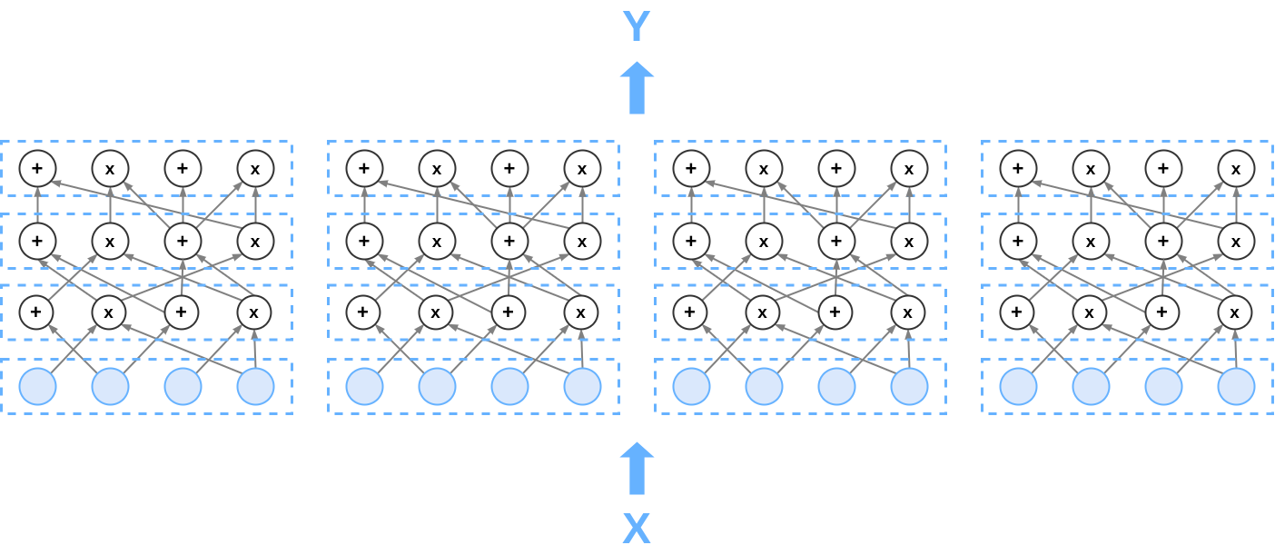
In what follows we will concern ourselves with arithmetic circuits C comprised of the side-by-side juxtaposition of N identical copies of the base circuit C_0. Thus C represents N parallel executions of the base circuit C_0.The circuit thus takes a vector x \in \mathbb{F}^{N \times G} as input and produces an output y \in \mathbb{F}^{N \times G}.

We’ll make some simplifying (but not strictly necessary) assumptions:

  • the width of the base circuit is the same at every layer,
  • in particular, inputs (x) and outputs (y) have the same size,
  • both G = 2^{b_G} and N = 2^{b_N} are powers of 2.

Arithmetization

The Gir++ protocol provides and argument for the relation: R_L = \Big\{(x, y) \in (\mathbb{F}^{N \times G})^2~\Big|~ y = C(x)\Big\}

Describing the protocol requires one to define a certain number of functions. These functions capture either the geometry of the circuit or the values flowing through it. To make matters precise, we consistently use the following notations for input variables

  • q'\in\{0, 1\}^{b_N} is the index of one of the N identical copies of the base circuit C_0 within C,
  • q\in \{0, 1\}^{b_G} is a “horizontal index” within the base circuit,
  • i\in [d]=\{0,1,\dots,d\} is a layer (“vertical index”) within the base circuit.

This makes most sense if one thinks of the subcircuit as a “matrix of arithmetic gates”. Thus a pair (q,i) describes the position of a particular arithmetic gate in the base circuit, and a triple (q',q,i) describes the arithmetic gate at position (q,i) in the q'-th copy of the base circuit C_0 within C.

  • h'\in\{0, 1\}^{b_N} represents the index of a copy of the base circuit within C
  • h_L,h_R\in\{0, 1\}^{b_G} represent two “horizontal indices” in the base circuit.

With that notation out of the way, we describe various functions. The first lot describes the circuit geometry. Recall that all gates are fan-in 2:

  • add_i(q, h_L, h_R) = 1 iff the gate q at layer i takes both h_L and h_R as inputs from layer i - 1 and is an addition gate. Otherwise add_i(q, h_L, h_R) = 0.
  • mul_i(q, h_L, h_R) = 1 if the gate q at layer i takes both h_L and h_R as inputs from layer i - 1 and is an multiplication gate. Otherwise mult_i(q, h_L, h_R) = 0.
  • eq(a, b) returns a == b

Next we introduce functions that captures the values that flow through the circuit:

  • V_i(q', q) is the output value of the gate at position (q,i) in the q'-th copy of the base circuit C_0 within C.

The \Bbb{F}-valued function below captures transition from one layer to the next:

  • P_{q', q, i}(h', h_L, h_R) = eq(h',q') \cdot \left[ \begin{array}{r} add_i(q, h_L, h_R)\cdot(V_{i-1}(q', h_L) + V_{i-1}(q', h_R))\\+\;mul_i(q, h_L, h_R)\cdot V_{i-1}(q', h_L)\cdot V_{i-1}(q', h_R)\end{array}\right].

It holds that V_i(q',q) = \sum_{h' \in \{0, 1\}^{b_N}}\sum_{h_L< h_R \in \{0, 1\}^{b_G}}P_{q', q, i}(h', h_L, h_R) This is not complicated to see: the RHS of this equation contains at most one nonzero term.

Key observation. V_i is expressed as an exponentially large sum of values of the function of V_{i-1}. The sumcheck protocol described in the next section provides polynomial time verifiable proofs for assertions of the form

\displaystyle\qquad\qquad\texttt{(some claimed value)} =\sum_{x\in\left\{\begin{array}{c}\text{exponentially}\\ \text{large domain}\end{array}\right\}}f(x)

for domains of a “specific shape” and “low degree” functions f:\Bbb{F}^n\to\Bbb{F}. This gives rise to a proof system for R_L.

The sumcheck protocol: setting up some notation

This section describes the sumcheck protocol. It is a central piece of how Gir++ works.

Multilinear polynomials are multivariate polynomials P(X_1,\dots,X_n)\in\Bbb{F}[X_1,\dots,X_n] that are of degree at most 1 in each variable. e.g.: P(U,V,W,X,Y,Z)=3 + XY + Z -12 UVXZ +7 YUZ (it has degree 1 relative to U,V,X,Y,Z and degree 0 relative to W). In general, a multilinear polynomial is a multivariate polynomial of the form P(X_1, X_2\dots, X_{d}) = \sum_{i_1 \in \{0, 1\}}\sum_{i_2 \in \{0, 1\}}\cdots\sum_{i_{d} \in \{0, 1\}} a_{i_1, i_2, \dots, i_{d}} \prod_{k=1}^{d} X_k^{i_k} with field coefficients a_{i_1, i_2, \dots, i_{d}}\in\Bbb{F}.

Interpolation. Let f: \{0,1\}^d \rightarrow \mathbb{F} be any function. There is a unique multilinear polynomial P_f=P_f(X_1,\dots,X_d) that interpolates f on \{0_\mathbb{F}, 1_\mathbb{F}\}^d. Call it the arithmetization of f. For instance P(X,Y,Z)=X+Y+Z-YZ-ZX-XY+XYZ is the arithmetization of f(x,y,z)=x\vee y\vee z (the inclusive OR).

In the following we will sometimes use the same notation for a boolean function f and its arithmetization P_f. This is very convenient as it allows us to evaluate a boolean function \{0,1\}^d\to\Bbb{F} on the much larger domain \Bbb{F}^d. This is key to the sumcheck protocol described below.

Partial sum polynomials. If P\in\Bbb{F}[X_1,\dots,X_d] is a multivariate polynomial, we set, for any i=1,\dots,d, P_i \in\Bbb{F}[X_1,\dots,X_i] defined by P_i(X_1, ..., X_i) = \sum_{b_{i+1}, \dots, b_d\in\{0,1\}} P(X_1,\dots,X_i,b_{i+1},\dots,b_d) the partial sums of P on the hypercube \{0, 1\}^{d-i}. We have P_d = P. Note that each P_i is of degree \leq \mu in each variable.

The sumcheck protocol: what it does

The (barebones) sumcheck protocol allows a prover to produce polynomial time checkable probabilistic proofs of the language R_L = \Big\{(f,a) ~\Big|~ f:\{0,1\}^d \rightarrow \mathbb{F} \text{ and }a \in \mathbb{F} \text{ satisfy } \sum_{x \in \{0, 1\}^d} f(x) = a\Big\} given that the verifier can compute the multilinear extension of f (directly or by oracle access). Verifier time is O(d + t) where t is the evaluation cost of P. The protocol transfers the cost of evaluating the P=P_f on the whole (exponential size) boolean domain to evaluating it at a single random point \in\Bbb{F}^d.

Note: the sumcheck protocol works more broadly for any previously agreed upon, uniformly “low-degree in all variables” multivariate polynomial P which interpolates f on its domain. The only important requirement is that P be low degree in each variable, say \deg_{X_i}(P)\leq \mu for all i=1,\dots,d and for a “small” constant \mu. In the case of multilinear interpolation of f one has \mu=1, but it can be useful (and more natural) to allow larger \mu depending on the context (e.g. GKR).

We actually need a variant of this protocol for the relation R_L = \left\{(f_1, f_2, f_3,a) ~\left|~ \begin{array}{l}f_1,f_2,f_3:\{0,1\}^d \rightarrow \mathbb{F} \text{, } a \in \Bbb{F}\\\text{ satisfy } \displaystyle\sum_{x \in \{0, 1\}^d} f_1(x)f_2(x)f_3(x) = a\end{array}\right.\right\}. This changes things slightly as we will need to work with multivariate polynomials of degree \leq 3 in each variable. To keep things uniform, we suppose we are summing the values of a single function f (or a low-degree interpolation P thereof) over the hypercube \{0,1\}^d which is of degree \leq \mu in all d variables. e.g. for us f=f_1f_2f_3, P=P_{f_1}P_{f_2}P_{f_3} and \mu=3. The sumcheck protocol provides polynomial time checkable probabilistic proofs with runtime O(\mu d + t).

The sumcheck protocol: the protocol

The sumcheck protocol is a multi-round, interactive protocol. It consists of d rounds doing ostensibly the same thing (from the verifier’s point of view) and a special final round.

At the beginning, the verifier sets a_0 := a, where a is the claimed value of the sum of the values of f (i.e. of a uniformly low-degree extension P of f) over the hypercube \{0,1\}^d.

Round 1

  • The prover sends P_1(X_1) (univariate, of degree at most \mu), i.e. a list of \mu+1 coefficients in \Bbb{F}.
  • The verifier checks that P_1(0) + P_1(1) = a_0.
  • The verifier randomly samples \eta_1\in\Bbb{F}, sends it to the prover and computes a_1 = P_1(\eta_1).

The next rounds follow the same structure.

Round i\geq 2

  • The prover sends P_i(\eta_1,\dots,\eta_{i-1},X_i) (univariate, of degree at most \mu), i.e. a list of \mu+1 coefficients in \Bbb{F}.
  • The verifier checks that P_i(0) + P_i(1) = a_{i-1}.
  • The verifier randomly samples \eta_i\in\Bbb{F}, sends it to the prover and computes a_i = P_i(\eta_i).

Giraffe describes a refinement to compute the evaluations of p_i in such a way the prover time remains linear in the number of gates: link to the paper. Libra also proposes an approach in the general case (meaning even if we don’t have data-parallel computation)

Special final round

The verifier checks (either direct computation or through oracle access) that P_{d}(\eta_{d})\overset?=P(\eta_1, \dots, \eta_{d}). In some applications it is feasible for the verifier to evaluate P directly. In most cases this is too expensive.

The sumcheck protocol reduces a claim about an exponential size sum of values of P to a claim on a single evaluation of P at a random point.

The GKR protocol

The GKR protocol produces polynomial time verifiable proofs for the execution of a layered arithmetic circuit C. It does this by implementing a sequence of sumcheck protocols. Each iteration of the sumcheck protocol inside GKR establishes “consistency” between two successive layers of the computation (starting with the output layer, layer 0, and working backwards to the input layer, layer d). Every run of the sumcheck protocol a priori requires the verifier to perform a costly polynomial interpolation (the special final round). GKR bysteps this completely: the prover-provides the (supposed) value of that interpolation, and another instance of the sumcheck protocol is invoked to prove the correctness of this value. In GKR, the only time the final round of the sumcheck protocol is performed by the verifier is at the final layer (layer d: input layer).

The key to applying the sumcheck protocol in the context of the arithmetization described earlier for a layered, parallel circuit C is the relation linking the maps V_i, P_{q', q, i} and V_{i-1} (here these maps are identified with the appropriate low-degree extensions). Establishing consistency between two successive layers of the GKR circuit C takes up a complete sumcheck protocol run. Thus GKR proofs for a depth d circuit are made up of d successive sumcheck protocol runs.

The main computational cost for the prover is computing intermediate polynomials P_i. This cost can be made linear if P can be written as a product of multilinear polynomials as decribed in Libra by means of a bookkeeping table.

First round

  • The verifier evaluates v_{d} = V_{d}(r_{d}', r_{d}) where (r_{d}', r_{d}) \in \mathbb{F}^{b_N + b_G} are random challenges. Then he sends r' and r to the prover. The evaluation of V_{d} can be done by interpolating the claimed output y.
  • The prover and the verifier engages in a sumcheck protocol to prove that v_{d} is consistent with the values of the layer d-1. To do so, they use the relation we saw previously. V_i(q',q) = \sum_{h' \in \{0, 1\}^{b_N}}\sum_{h_L,h_R \in \{0, 1\}^{b_G}}P_{q', q, i}(h', h_L, h_R)

Important note. This is an equality of functions \{0,1\}^{b_N}\times\{0,1\}^{b_G}\to\Bbb{F}:

  • on the LHS the map V_i(\bullet',\bullet)
  • on the RHS the map \sum_{h' \in \{0, 1\}^{b_N}}\sum_{h_L,h_R \in \{0, 1\}^{b_G}}P_{\bullet', \bullet, i}(h', h_L, h_R)

Since we are going to try and apply the sumcheck protocol to this equality, we first need to extract from this equality of functions an equality between a field element on the LHS and an exponentially large sum of field elements on the RHS. This is done in two steps:

  • multilinear interpolation of both the LHS and RHS to maps \Bbb{F}^{b_N}\times\Bbb{F}^{b_G}\to\Bbb{F},
  • evaluation at some random point (Q',Q)\in\Bbb{F}^{b_N}\times\Bbb{F}^{b_G}
  • sumcheck protocol invocation to establish V_i(Q',Q) = \sum_{h' \in \{0, 1\}^{b_N}}\sum_{h_L,h_R \in \{0, 1\}^{b_G}}P_{Q', Q, i}(h', h_L, h_R), which requires low degree interpolation of the map P_{Q', Q, i}(\bullet', \bullet_L, \bullet_R):\{0,1\}^{b_{N}}\times\{0,1\}^{b_{G}}\times \{0,1\}^{b_{G}}\to\Bbb{F}. This particular low degree-interpolation is systematically constructed as a product of multilinear interpolations of functions that together make up the map P_{\bullet', \bullet, i}(\bullet', \bullet_L, \bullet_R):\{0,1\}^{b_{N}}\times\{0,1\}^{b_{G}}\times\{0,1\}^{b_{N}}\times\{0,1\}^{b_{G}}\times \{0,1\}^{b_{G}}\to\Bbb{F}

We won’t bother further with the distinction (q,q')\in\{0,1\}^{b_N}\times\{0,1\}^{b_G} and (Q,Q')\in\Bbb{F}^{b_N}\times\Bbb{F}^{b_G}.

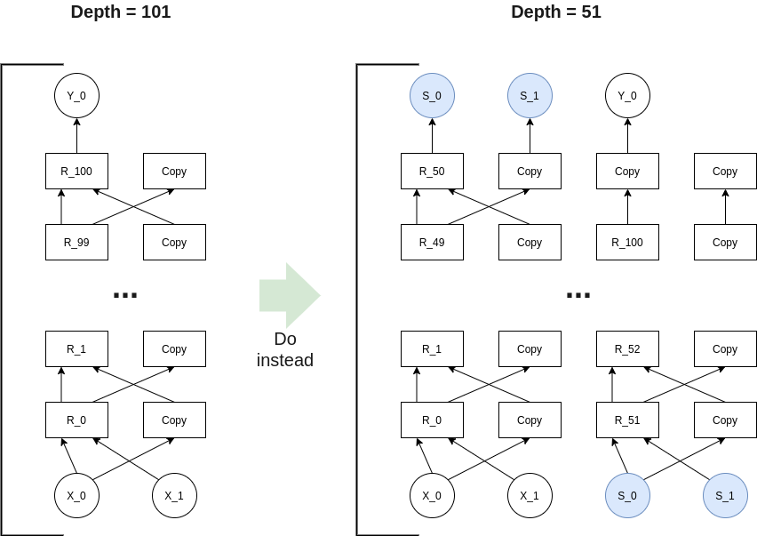
As a result, at the final round of the sumcheck, the verifier is left with a claim of the form P_{r_{d}', r_{d}, i}(r'_{d-1}, r_{L, d-1}, r_{R, d-1}) == a, where r'_{d-1}, r_{L, d-1} and r_{R, d-1} are the randomness generated from the sumcheck. Instead of directly running the evaluation (which requires knowledge of V_{d-2}), the verifier asks the prover to send evaluation claims of V_{d-1}(r'_{d-1}, r_{L, d-1}) and V_{d-1}(r'_{d-1}, r_{L, d-1}). The verifier can then check that those claims are consistent with the claimed value of P_{r_{d}', r_{d}, i} using its definition.

To sum it up, we reduced a claim on V_{d} to two claims on V_{d-1}.

Intermediate rounds

We could keep going like this down the first layer. However, this would mean evaluating V_0 at 2^d points. This exponential blow up would make the protocol impractical. Thankfully, there are two standard tricks we can use in order to avoid this problem. Those are largely discussed and explained in the Hyrax and Libra paper.

  1. The original GKR paper asks the prover to send the univariate restriction of V_i to the line going through v_{0, i} and v_{1, i} and use a random point on this line as the next evaluation point.
  2. An alternative approach due to Chiesa et al. is to run a modified sumcheck over a random linear combination \mu_0 P_{q', q_0, i} + \mu_1 P_{q', q_1, i}. By doing this, we reduce the problem of evaluating V_i at two points to evaluating V_{i-1} at two point. It is modified in the sense that the “circuit geometry functions” add_i and mul_i are modified from round to round:
    \begin{array}{l}(\mu_0 P_{q', q_0, i} + \mu_1 P_{q', q_1, i})(h', h_L, h_R) \\ \quad= eq(q', h')\cdot \left[\begin{array}{c}(\mu_0add_i(q_0, h_L, h_R)+\mu_1add_i(q_1, h_L, h_R))\cdot(V_{i-1}(h', h_L)+V_{i-1}(h', h_R)) \\[1mm]+ (\mu_0mul_i(q_0, h_L, h_R)+\mu_1mul_i(q_1, h_L, h_R))\cdot V_{i-1}(h', h_L)\cdot V_{i-1}(h', h_R)\end{array}\right]\end{array} The overhead of this method is negligible.

Hyrax and Libra suggest to use the trick (2) for the intermediate steps. For the last rounds, we will instead apply the trick (1). This is to ensure that the verifier evaluates only one point of V_0.

The last steps

At the final steps, the verifier evaluates V_0 at the point output by the last sumcheck.

Cost analysis

As a sum up the verifier:

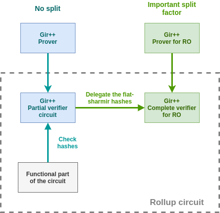
  • Generate the first randomness by hashing (x, y). One (|x| + |y|)-sized hash. In practice, this computation is larger than all the individual hashes. We expand later on a strategy making this practical.
  • Evaluates V_{d} and V_0 at one point each.
  • d(2b_G + b_N) consistency checks. As a reminder they consists in evaluating a low-degree polynomial at 3 points: 0, 1, \eta. And calling a random oracle.

For the prover

  • Evaluate the V_k. This is equivalent to execute the computation.
  • Compute the polynomials of the sumcheck: ~\alpha dNG + \alpha dGb_G multiplications, where \alpha is small (~20). Since, in practice N \gg b_G, we can retains 20dNG.
  • d(2b_G + b_N) fiat-shamir hashes to compute
8 Likes

Our contribution (2/2)

Having recalled the basics of sumcheck and GKR, we are ready to present our idea. We stress that this is a proposal. We are very interested in receiving feedback, in particular attempts at breaking this scheme.

Compiling GKR verifier in a R1CS

Hyrax proposes to compile this protocol using discrete-logs assumptions in order to obtain a zero-knowledge succinct non-interactive argument of knowledge. Its purpose is to establish a proof system without trusted setup. Libra propose to use a multilinear commitment, this encapsulate the evaluations of V_d and V_0 at the expense of an increased prover time.

The verifier typically runs in ~1sec. However, it is be feasible to check the verifier transcript of the GKR NIZK with a pairing-based argument (like Plonk or Groth16).

The evaluations of V_0 and V_{d} requires few multiplication gate: 1 for each input and 1 for each output. On top of that it allows us to check relations between the inputs and the output cheaply. And the verifier time is constant.

The sumchecks are however expensive to verify in practice as we need to use randomness from the verifier. The classical way to do it non-interactively is to use the Fiat-Shamir heuristic and therefore a hash function. Even though, this is a logarithmic overhead, it has a large constant (in our circuit, we need to hash ~20k field elements).

Tuning GKR to make it a gMIMC hash proving accelerator

In the constraints model of GKR we may only have addition gates and multiplication gates and we cannot use “constants”. However, nothing prevents us from using different sets of gates. One may even use gates with different fan-in if needed. We take advantage of this observation to design a proof system specially tailored for data-parallel gMIMC hash computation. Each copy of the base circuit takes 2 inputs and returns one output.

Using custom gates

Following a suggestion in Libra, we define a custom family of gates. Let \alpha be the exponent for gMiMC in \Bbb{F} (a small positive integer, 3 - 7 in practice) and let k(1),\dots,k(101) be elements in \mathbb{F} (there are 101 rounds in gMiMC). Ciph_{k(i), \alpha}(x,y) = x + (y + k(i))^\alpha and the copy gate Copy(x, y) = x

The polynomial P_{q', q, i} must be set to P_{q', q, i}(h', h_L, h_R)= eq(q', h')\cdot\left[\begin{array}{r}ciph_i(q, h_L, h_R)\cdot Ciph_{k(i), \alpha}\Big(V_{i-1}(h', h_L),~V_{i-1}(h', h_R)\Big) \\+ copy_i(q, h_L, h_R)\cdot Copy\Big(V_{i-1}(h', h_L),~ V_{i-1}(h', h_R)\Big)\end{array}\right] The ciph_i(\bullet, \bullet_L,\bullet_R) and copy_i(\bullet, \bullet_L,\bullet_R) functions are the analog of the add_i(\bullet, \bullet_L,\bullet_R) and mul_i(\bullet, \bullet_L,\bullet_R) in that they encode the geometry of the gMiMC base-circuit. We use multilinear interpolation to extend their domain. For cost analysis (see below) we record the degrees of these polynomials w.r.t. the variables:

  • it has degree \alpha+1 in h',
  • it has degree 2 in h_L
  • it has degree \alpha + 1 in h_R.

(Note: the various “+1” and “+2” come from degree 1 occurrences of variables in eq, ciph_i and copy_i.)

The verifier has to evaluate a degree \alpha polynomial in the consistency checks of the sumcheck. Since alpha is small, this is a negligible overhead compared to the cost of hashing. We can also still use Libra’s bookkeeping algorihm to keep the prover runtime small.

As a result, we obtain a GKR circuit able to verify the computation of N = 2^{b_N} hashes. Its base circuit consists of 2 gates per each layer (one copy gate, one ciph gate) and has a depth of 101.

Summing up, the consistency check costs 101[(b_N + 1)(\alpha + 2) + 3] constraints. The cost of Fiat-Shamir hashing is, for each GKR layer, (\alpha + 2) hashes of field elements: b_N times for the sumchecks rounds on h', \alpha + 2 field elements once for those on h_R and 3 fields elements once for those on h_L. Let T(n) denote the cost of hashing a string of n fields elements. The total cost of the Fiat-Shamir hash can be rewritten as 101[(b_N + 1)T(\alpha + 2) + T(3)]. These hashes could conceivably be computed directly in the smart contract using a cheap hash function (b_N=20, \alpha=7 equate to 20k hashes and a multiexp of that size or inside the SNARK) or inside the SNARK circuit (with approximatively T(n) = 350n, we estimate it is going to cost an additional 7M constraints.

The evaluation of V_0 and V_{d} is efficient in term of constraints. We need to interpolate 2 multilinear polynomials at given points from their evaluation representation. It takes 1 constraint per input and 1 constraint per output for a total of 3N constraints (plus the logarithmic overhead) per hash to prove. We can similarly obtain circuits for proving hashes with a different number of inputs using analogous methods.

Splitting the depth of the circuit

Although the circuit is asymptotically efficient, the sumcheck induces a lot of overhead, mostly because of the Fiat-Shamir hashes. It is possible to trade asymptotic efficiency for lower overhead by using two sub-circuits of depth 51 to compute a hash. This implies that each sub-circuit is doing two halves of the rounds needed to compute a hash in parallel. Hence a two-fold decrease of depth but a two-fold increase in size of the public input/output. This can be generalized for any n-split of the circuit.

Composing several GKR circuits

As already mentioned, the majority of the verifier overhead lies in the usage of Fiat-Shamir to generate the sumcheck’s challenges. Depending on the input size, it yields in practice the need to hash 10000-30000 field elements. We propose to delegate the hashes to another GKR circuit with an important split factor.

As a result, the rollup circuits has less hashes to perform which contribute to the reduce the overhead.

Generating the initial randomness

There remains an unsolved problem: generating the very first random input r_1 for the very first round of the very first sumcheck run dedicated to checking consistency between layers 0 and 1. In an interactive setting, this would pose no problem: the verifier would simply randomly sample r_1=(q_1',q_1)\in\Bbb{F}^{b_N}\times\Bbb{F}^{b_G}, send it to the prover who would then start work on generating a sumcheck proof for the equality
V_d(r_1) = \sum_{h\in\{0,1\}^{b_N}}\sum_{h_L,h_R\in\{0,1\}^{b_G}} P_{q',q,d}(h, h_L,h_R), and continue down the sumcheck protocol. When we turn things non-interactive, though, we need to efficiently generate the initial randomness, verifiably and with little overhead. Of course, hashing all of x and y (say) is out of the question: this is precisely the work that the verifier tries to avoid having to do. We see three viable possibilities for that.

  • Generate randomness from a separate deterministic sumcheck / GKR run
  • Pedersen Hash solution

Generate randomness from a separate deterministic sumcheck

Both a (noninteractive) sumcheck run and a (noninteractive) GKR run involve moderate hash computations. To be precise: under Fiat-Shamir, every variable elimination, i.e. every round in the sumcheck protocol, as well as the final round, require a hash computation.

The idea is thus to do a separate run (of either a new sumcheck problem or the actual GKR) using an initial random seed (likely low entropy and possibly biasable). That separate run is used to bind us to x and y through intermediate Fiat-Shamir hash computations. Note taht this involves only very few intermediate hashes. Using the hashes thus produces, one constructs a good initial random seed for the actual circuit verification.

In other words, one uses a dummy sumcheck / GKR run to produce a quickly (polynomial time) verifiable hash for an (exponentially) large input (x and y). Since the SNARK circuit re-uses x and y in the actual GKR proof, we expect this to be binding to x and y.

We see three simple ways to generate an agreed upon initial seed:

  • a hardcoded value such as r_1^\mathsf{sep}=-1, or a “more complicated” hardcoded value r_1^\mathsf{sep}\in\Bbb{F} (e.g. a generator of \Bbb{F}^\times).
  • a value r_1^\mathsf{sep} deterministically generated from a random beacon value RB that changes periodically and is known to all participants

We next describe two options for the separate sumcheck / GKR runs used to generate the initial randomness.

A simple sumcheck

Let r_1^\mathsf{sep} be some agreed initial randomness seed. One can consider the following sumcheck problem a=\sum_{i=1}^{G\times N}x_i+\sum_{i=1}^{G\times N}y_i=\sum_{i=1}^{2\times G\times N}u_i where we set u=x\|y, the concatenation of the vectors x and y, and view it (equivalently) as a function \widehat{u}:\{0,1\}^{b_G + b_N + 1}\to\Bbb{F} where \widehat{u}\big(\epsilon_0,\dots,\epsilon_{b_G+b_N}\big)=u_i if \epsilon_{b_G+b_N}\cdots\epsilon_1\epsilon_0 is the binary representation of i-1\in[\![~0\dots 2^{b_G+b_N+1}~[\![ for instance.) Alternatively, one may also consider u'=x\|0_{G\times N}\|y\|0_{G\times N} or some other padded variant on u (again, viewing it as a function \widehat{u'}:\{0,1\}^{b_G + b_N + 1 + 1}\to\Bbb{F}. Padding with 0’s (and thus doubling the size of the domain of the function) doesn’t affect the sum but produces an extra round in the sumcheck protocol and completely changes the intermediate steps of the computation.

Using the (low entropy) initial seed r_1 as the initial randomness for Fiat-Shamir, one runs an instance of sumcheck computing intermediate hashes as one goes along. The intermediate hashes thus generated (O(b_G+b_N) many) serve as binding commitments to x and y. From them, one is free to deterministically generate the proper randomness r_1 to be used to bootstrap the actual Fiat-Shamir noninteractive execution of GKR.

Note that x and y will (likely) be private inputs in the Snark circuit. (Although they may be public for some use cases, or parts of them may be public, for instance if the overall computation represents Merkle branch verifications from leaves to a public root hash.) Thus the Snark circuit will re-use these same x and y in the proper GKR verification.

Duplicating the GKR run

The idea is the same as above, but rather than using a completely different instance of the sumcheck protocol to generate the randomness bootstraping the “real” noninteractive GKR verification, one runs a dummy verification of the same GKR circuit (with initial randomness r_1^\mathsf{sep}).

Again, the SNARK circuit will ensure that x and y are re-used in both executions. This demands more work from the prover in that it doubles the effort on the prover’s end (and only slightly more work from the verifier). But it produces further consistency. Indeed, the first polynomial produced in the GKR prover run, P_1(X_1)=\sum_{b_2,\dots,b_n\in\{0,1\}} P(X_1,b_2,\dots,b_n), is the same no matter what. Its coefficients (of which there are very few, say, 3\mu) may thus be provided as further public data in the SNARK circuit used to verify the GKR proof.

N.B. We believe the first solution (separate sumcheck run) to be just as safe and less work for the prover, and thus superior.

Pedersen Hash solution

All of the checks we describe live in a constraint system. This approach proposes to leverage the final verifier in order to succinctly prove the hashing of x and y. We do it with the following protocol transforms:

  • Make x and y public inputs of the SNARK proof (if they were not already, it depends on the use-case). We set u = x \| y, the concatenation of the vectors x and y, and set u_i to be its i-th coordinate.

A priori this would require the prover to send x and y to the verifier, who would have to include them in its SNARK multi-exponentiation. For large computations (i.e. large vectors x and y) this imposes a large multi-exponentiation onto the verifier, which is undesirable. Furtermore, the verifier may not care about either x and y, say if they represent intermediate steps in a Merkle proof where only the root hash is public knowledge (and thus, ideally, only the last coordinate of y, say, ought to be public data). This problem is bypassed as follows.

  • The prover computes G = \sum_{i \in [|u|]} u_i\cdot G_i, where the G_i are the SNARK verification key parts corresponding to the public inputs u_i, and sends it to the verifier.

The verifier thus won’t need to compute the associated part of the public input multi-exponentiation. It can directly plug G into the multi-exp. The purpose fo G is to be binding to x and y and to serve as the randomness seed for the very first Fiat-Shamir randomness.

  • Both the verifier and prover compute r = H(G).

We upgrade r to a public input of the SNARK proof. There is thus an associate curve point G_r in the verification key to be used by the verifier in its multi-exponentiation. The purpose of r is to serve as the initial Fiat-Shamir randomness.

  • The verifier computes its public input multi-exponentation as r\cdot G_r + G + \Delta where \Delta is the remaining part of the multi-exp, corresponding to the “actual SNARK verification”.

This is equivalent of the using the hash of a pedersen hash of x and y by reusing the trusted setup. It is worth noting that in the end, the verifier does not have to perform computation linear in |u| as the prover does it for him.

9 Likes

Summarizing my own intuition pumps for this scheme below.

Let’s take a much simpler example, where the circuit is just the raw MIMC permutation: x_{i_1} = x_i^3 + k_i. So each “copy” of the circuit is just a straight line, of depth d (eg. d = 200). Let V_0(b_1...b_k) be a k-variate linear-in-each-variable polynomial representing a “hypercube” containing the inputs (ie. the inputs would be at V_0(0, 0, 0...0, 0), V_0(0, 0, 0...0, 1), V_0(0, 0, 0...1,0) etc) and V_d(b_1....b_k) is similarly a polynomial representing a hypercube containing the outputs.

Within the hypercube (ie. at all inputs where all coordinates are 0 or 1), we have V_{i+1}(b_1...b_k) = V_i(b_1...b_k)^3 + k_i. But we can’t make this true for the polynomials in general (ie. including outside the hypercube), because then the degree of each V_i would keep multiplying by three, so later V_i's would take an exponential amount of time to compute (and require an exponentially large trusted setup). Rather, we want each V_i to be linear in each variable. So instead, we pull some clever tricks involving sumcheck protocols.

Let us define the polynomial eq(b_1...b_k, c_1...c_k) as being the multilinear polynomial that equals 1 when (c_1 ... c_k) = (b_1 ... b_k) and 0 elsewhere inside the hypercube. For example, for k = 2, the polynomial would be:

(1-b_1) * (1-b_2) * (1-c_1) * (1-c_2)
+ (1-b_1) * b_2 * (1-c_1) * c_2
+ b_1 * (1-b_2) * c_1 * (1-c_2)
+ b_1 * b_2 * c_1 * c_2

We now make a new equation connecting V_{i} and V_{i+1}:

V_{i+1}(b_1...b_k) = \sum_{(c_1...c_k) \in \{0,1\}} eq(b_1...b_k, c_1...c_k) * V_i(c_1...c_k)^3 + k_i

If you evaluate this equation for any point (b_1...b_k) in the hypercube, you’ll get an expression that contains V_i^3 + k in one term (where (c_1...c_k) = (b_1...b_k)) and zero everywhere else. Now you might ask, why do this? Why make the relation even more complicated by turning it into a sum containing the original value plus a bunch of zeroes?

The answer is this: unlike the original equation V_{i+1}(b_1...b_k) = V_i(b_1...b_k)^3 + k_i., which is only true inside the hypercube, this new equation is true everywhere; one could evaluate it at V_{i+1}(123, -5, 42069, 7395723240) and it would check out, despite the fact that V_{i+1} or even eq don’t directly “mean anything” at those coordinates.

Notice a key piece of cleverness that makes this possible: no matter which point you’re evaluating V_{i+1} at, V_i is only ever evaluated within the hypercube. The randomization in making an “out-of-domain” evaluation instead comes from the fact that if you try to evaluate the above expression outside the hypercube, it’s eq that will give outputs other than 0 or 1, and so you’re doing a random-looking linear combination across the whole domain.

Now, how do we actually use this? First, recall the sum-check protocol:

  • You are trying to prove a_0 = \sum_{b_1...b_k \in \{0,1\}} f(b_1...b_k)
  • You provide P_1(0) = \sum_{b_2...b_k \in \{0,1\}} f(0, b_2...b_k) (ie. the top half of the cube) and P_1(1) = \sum_{b_2...b_k \in \{0,1\}} f(1, b_2...b_k) (ie. the bottom half of the cube)
  • Verifier sends you a random coordinate r_1, computes a_1 = P_1(r_1), and asks you to recursively prove \sum_{b_2...b_k \in \{0,1\}} f(r_1, b_2...b_k) (one can think of this as taking a random linear combination of the top and bottom halves of the cube, and repeating the protocol with the resulting half-size cube)
  • Repeat until the prover provides the constant P_n = f(r_1 ... r_k). Use the original polynomial commitment to f to verify that this evaluation is actually correct.

We use this protocol, but we do something clever. We start by asking for a commitment to V_0 and V_d, take a random coordinate z_d = (b_1 ... b_k), ask for V_d(z_d). The goal is, of course, to prove that the above sum-check relation holds between V_d and V_{d-1}, V_{d-1} and V_{d-2} and so on all the way down to V_1 and V_0. But to save prover time we’re not going to ask the prover to make a commitment to any of the intermediate V_i layers. Instead, we run the sumcheck protocol for V_d(z_d), get out of it some point z_{d-1} = (r_1...r_k), and we directly plug that into the sumcheck protocol for the next layer. We keep walking through all the layers, and finally we get a claimed evaluation of V_0, and we check that against V_0. Effectively, we don’t even bother checking anything in the middle, we just trust the prover all the way until the circuit gets to an evaluation of V_0, and only check its correctness at the end.

This allows you to prove N MIMC permutations with commitments (ie. size-N polynomials, requiring a size-N elliptic curve linear combination) at only the start and the end, so you only need 2N elliptic curve operations. Everything in the middle only requires prime field operations, which are much faster. You can then use the V_0 and V_d commitments as a lookup table in PLONK, accessing the table in one constraint per read.

The work above extends this scheme to look at not just homogeneous circuits that repeat circuits of width 1, but also repeated circuits more generally.

8 Likes

Very cool!

One issue with GKR-based protocols including Giraffe, Libra, Gir++ etc. is that they require layered arithmetic circuits. Also, the verifier’s proof checking scales with the depth of the layered circuit (so hundreds of layers for MiMC).

Check out an adaptation of the sum-check protocol and multilinear polynomials that avoids these problems in the Spartan proof system: https://eprint.iacr.org/2019/550.pdf. I suspect Spartan can also support parallel computation (see SpartanNIZK).

2 Likes

Spartan is brilliant and we were aware of it.

However, in our use-case (fast prover) we want to have as little cryptographic operations as possible. The great benefit of layered arithmetic circuits is that the intermediate-layer-witness-values are swallowed up by the sumchecks. Thus only the inputs and the outputs are subject to cryptographic operations (e.g. commiments). In Spartan, however, and more generally in any R1CS based scheme it seems, you need to commit to the entire witness.

On top of this, the number of GKR rounds you do only incurs a logarithmic time cost for the verifier (in the number of hash you prove, for a constant hash function). So, in a use-case where you want to check plenty of hashes it becomes negligible. The verifier runtime is dominated with the input-output checks.

1 Like

Got it! Yes, commitment to entire witness is indeed required.

Regarding GKR rounds, I might be misremembering details, but would one not need a separate sum-check for each layer in the circuit, how do you make the number of rounds logarithmic i.e., only log{circuit_width} rather than d * log{circuit_width}, where d is the depth of the circuit?

No, you are right. I meant the depth of the circuit is constant in the number of hash you check. Having a deep circuit results in a large constant in the verification time, but let’s view it from this angle.

You want to convince a verifier that you ran N instances of a circuit C of depth d and width W (assumed constant here), on input X and that you got output Y. You can let him do it trivially (run the computation yourself), it’s gonna take Z = O(dNW) operation for the operator. If you do a GKR proof, it’s gonna cost him A = O(NW) operation for the multilinear polynomial evaluation and (as your said) B = O(d * log(NW)). So no matter how big you pick d (and W), there is always a value of N that makes B / Z as small as you want. But of course, this only works in a context like rollup where you try to make proofs for as many statement as possible.

Thanks! Your analysis is spot on!

One additional question: how big is the satisfying assignment size (in the context of R1CS representation of Rollup circuits) with respect to the witness size (i.e., the size of input to layered arithmetic circuits, which for Rollup I believe would be a set of Merkle proofs)? I ask this because if that ratio is indeed large, the savings from layered circuits would indeed be substantial.

It is also worth considering the blowup in circuit size when building layered circuits as opposed to R1CS.

In the context of layered circuits, the saving ratio would be “#Gates in the inputs and output layers” / “#Gates in total in the circuit”. In our case: with gMIMC, (although it does not depends on the hash function you use, as long as you can model the hash function with a layered circuit) it’s ~200 (hence the claim).

It is also worth considering the blowup in circuit size when building layered circuits as opposed to R1CS.

What do you mean by the blowup in circuit size ?

While “#Gates in the inputs and output layers” / “#Gates in total in the circuit” is a great metric, we should also consider another metric:

  • #Gates in total in the layered circuit”/ “#constraints in the R1CS encoding of Rollup”. I hope this is close to 1, otherwise this will eat away savings from the use of layered sum-check. I’m not sure about Rollup computation but this ratio could be anywhere from 2 to ~100 (in degenerate cases) depending on the computation.

This is what I meant by blowup in circuit size.

Oh right, hard to answer and for several reasons:

  • In GKR as we use it, we can use custom gates (a little like turbo-plonk), so depending on your customization you may get a different ratio. It does not come for free, but there is always ground for optimization on that side.

  • Layered Circuits are less expressive than R1CS: you cannot express everything you want in the form of a layered circuit. For instance, (in my knowledge) you can’t decompose an inputs into bits without putting each bit value in the input vector. That’s why I believe this kind of scheme can only be used for very specific use cases. I have wondered if we could use GKR for signature verification, but I don’t think this is possible because of this as well.

  • However, provided that what you want to encode something that can be encoded in a layered circuit, you may experience a blowup if your computation uses a lot of linear combination/addition because of the fan-in limitation of GKR. But just like for custom gates, that’s something you can tune (not for 100% free)

EDIT: But since GKR only uses hash function, you can always embed the verifier in a R1CS (as suggested in the post). In that case the ratio only concerns the prover time, and it would be something like.

C_{\text{layered io}} + \alpha C_{\text{layered total}} vs {C_{\text{R1CS}}} where the \alpha is a very small constant that reflects the fact the GKR prover is an order of magniture faster than pairing-based SNARKs. However, the exact value of \alpha depends on the type of gates you use (and their degree), and this metric does not take into account the depth of the circuit.

  • Yes, that is true, custom gates could improve expressiveness at some cost.
  • That is my understanding as well. One would also need “bit tests” in the circuit to make sure the claimed bit element in the input is really either 0 or 1. While this is possible to do, it would make the circuit to be bigger since the result of bit tests must somehow show up in the circuit’s outputs either one output per bit test or compressed using randomness (where one random element per bit test would show up in the inputs). There may be ways to improve this, but that would require moving toward Spartan-style sum-check or similar. My understanding is Rollup computation needs to do signature verification. What is the plan for this?
  • Totally agreed on the third bullet.

The problem of embedding a Spartan-style proof verifier (only the computer-theoric part of it) into another proof system’s R1CS is that it has no benefit compared to simply doing the computation. If we could accelerate the proving time for any R1CS by a factor of several hundred compared to the current technics (similarly to what we propose with GKR), it would be a game-changer. However, I don’t know yet how to do that.

For signature, the “standard” approach is to use EDDSA a recursive curve like Jubjub/BabyJubjub as suggested by ZCash. The constraint cost is not too crazy (~4000 constraints if I am correct).
Or, you can use [BMMV19] Section 9, but it requires using the BLS signature scheme along with either a pairing-friendly recursive curve (like BLS12-377/BW761/MNT46) or Plookup. But I am not sure this will actually be faster when embedded in a R1CS.

Yes, I’m familiar with embedding ECDSA as a circuit and then use SNARK, but I was wondering how you plan to do signature verification using a different proof system and combine with GKR for hash circuits. I suppose you would somehow need to combine leaf nodes of the Merkle tree in the input layer of GKR with proofs about signature in a different proof system (e.g., bellman/groth16)?

I had one more question: is there a proof that that randomness generation strategy you described above is safe? If the prover knows the initial seed, can it not cheat by forging false proofs? Shouldn’t challenges in each round of the sum-check be generated from a random function for security?

The “use a dummy sumcheck/GKR round with weak initial randomness” approach to generating the initial randomness for the actual GKR run is flawed and can be attacked. We describe such an attack below.

  • Perform an honest dummy sumcheck/GKR round using the actual input / output vectors x / y.
  • Use the randomness r thus generated to boostrap the actual GKR run.
  • Rembember all the intermediate prover generated polynomials P_i, value functions V_i thus generated for both the dummy run and the actual GKR run.
  • Devise alternative input / output vectors x' and y' that will pass precisely the same sequence of sumcheck runs.
    The main observation now is that alternative vectors x' and y' satisfying (x',y')\neq(x, y) and which satisfy the system of constraints associated with the P_i, V_i, the underlying circuit and r will exist and be explicitely computable using tools from linear algebra. Indeed, every constraint depends linearly on x' and y'. Thus every such constraint shaves off at most one dimension from the solution space. If (x,y)\in\Bbb{F}^{2NG}, this produces a solution space of pairs (x',y') of dimension at least 2NG-(b_N+b_G+1+O(b_N)) where b_N+b_G+1 constraints arise from the dummy sumcheck, and O(b_N) from the ensuing GKR protocol.
    Such attacks can be carried out even with the further imposition that some of the coordinates of x and y be public (e.g. they represent the current state root hash of a roll-up). Indeed any one such constraint may only reduce the dimension of the solution space by 1.

This attack does not work against the Pederson hash method. If we could produce a collisions in (essentially) (x,y)\mapsto \sum_i^N (x_i [s^i G] + y_i [s^{i+N} G]) we could extract s as one of the roots of \sum_i^N x_i T^i + y_i T^{i+N}.

1 Like

Thanks OliverBBB!

Above, there is a claim “If we could accelerate the proving time for any R1CS by a factor of several hundred compared to the current technics (similarly to what we propose with GKR), it would be a game-changer.”

What is the intuition for several 100x improvement? Sum-checks require multiple tens of field operations per gate (which could only be at most 10x cheaper than multiexp). From looking at Hyrax and Libra papers’ benchmarks reported, I don’t see how sum-checks can be 100x cheaper than say G16 prover. Have you analyzed this more rigorously?

I am not really sure how you get those numbers but the sumcheck takes 8N + 2(\alpha + 3)\frac{N}{2} = 28N field multiplication where N is the number of gates in the layer (using Libra’s bookkeeping method). On the other side a 256 bits elliptic curve multiplication take ~5000 field multiplications, and around 3 times more on G2. Even with the most efficient multiexp algorithm this would not compete. Also, note that Hyrax and Libra use cryptographic commitments to make their schemes succinct. This impacts the prover runtime and explains why you can’t see this much improvement on their benchmark data.

1 Like

On the other side a 256 bits elliptic curve multiplication take ~5000 field multiplications

I think those numbers actually do sound like it would be a 10-20x improvement. With fast linear combination algorithms, ECMULs are ~10 times faster batched than they would be independent, so it would still be ~500 field muls per ECMUL. And I have the feeling that 5000 is an overestimate; verifying EC addition steps is easier than computing them because all you need to do is prove that three points are (i) all on the curve, and (ii) on the same line. The latter is just a dot product where one vector is rotated 90’: (y_2-y_1)*(x_3-x_1) - (x_2-x_1)*(y_3-y_1) = 0. So all in all a 10x improvement seems reasonable.

That’s right if you think about verifying an ECMUL in a circuit. In that context, it would cost ~2000 constraints (but for an edward curve). However, note that you wouldn’t be able to use the fast multi-exponentiation algorithm in the circuit (because of the combinatoric etc…).

By 5000 , I mean the number of operation you have to do (as the prover) to perform an exponentiation (even though I agree that this is reduced in practice by the the fast-linear combination/multiexp algo). I rechecked my computation using this: here and got a average case of 256 * (7M + 3S) + 128 * (12M + 2S) = 3328M + 1024S. That’s where the x5000 came from. And once again all of this is hold for G1 but as a prover you also have to do G2 operations, and they are more expensive. Possibly, the x100 is overestimated but this is closer to x50 than x10. Also, the 28N holds for BN256’s gMIMC7, you would get 14N with BLS.

I guess we need an implementation and proper benchmark data if we want to clearly sort out the performance.

1 Like