by Fei Wu - This work was conducted during my internship at the EF. I thank my mentor @misilva73 for valuable discussions, feedback, and comments.
Overview
Under EIP-7999, execution, data, and state have separate gas targets, limits and base fees. These resource markets are nevertheless coupled. Runtime block-level access lists (BALs) consume data gas, but they are generated by execution and state activity. In this previous analysis, we model that a higher data base fee raises the BAL-inclusive price of those parent activities, reducing execution and state demand and, in turn, the BAL they generate.
This analysis solves the resulting joint equilibrium for the three resource dimensions. For each resource, equilibrium requires either that usage reaches its target at a base fee of at least 1 wei, or that the base fee reaches its 1-wei minimum and the resource underfills. We first ask whether an all-target-clearing equilibrium exists for a proposed combination of execution, data, and state targets. When the target-filling calculation would require an execution base fee below 1 wei, that target combination is not jointly supportable: execution instead becomes fee-floor-bound and settles below its configured target.

A flowchart showing how each resource is modeled. Execution and state demand respond to parent prices that include their runtime-BAL data charge. Realized parent activity determines execution gas, state gas, and runtime BAL; static data and runtime BAL then combine into total data-gas usage. The three resource markets jointly satisfy their target-clearing and one-wei minimum conditions.
This condition defines an execution-clearing boundary in execution/data target space. The boundary answers two equivalent capacity-design questions:
- for a given data target, what is the largest execution target that can be fully utilized while the execution base fee remains at or above 1 wei?
- for a given execution target, what is the minimum data target required for all three resources to clear?
The analysis combines resource-demand elasticities and metering multipliers established in resource elasticity and Glamsterdam equilibrium analysis with the static-data meter, runtime-BAL anchor, and BAL-inclusive parent-price model established in Data metering and BAL demand report.
The results serve as conditional equilibrium benchmarks rather than final protocol recommendations. They identify which parameter combinations are internally consistent under the modeled demand system and provide equilibrium operating points for the next stage of dynamic analysis.
The results presented in this post can be reproduced from this repository. Unless stated otherwise, the report assumes the following reference parameterization:
- Central elasticities are derived from the 35-day window around gas limit increase events, i.e., \epsilon_{\mathrm{execution}} = 0.121, \epsilon_{\mathrm{data}}=0.229, \epsilon_{\mathrm{state}} = 0.335.
- Co-produced state access from state-creating transactions follows execution activity, i.e., \lambda=0.
- State access intensity does not change as execution scales, i.e., \rho_A=1.
- Blob-linked reserve price for data gas is not considered.
Main results
- The execution-clearing boundary is the central design object. For each data target, it gives the maximum execution target that can clear before execution base fee reaches 1 wei. In the reference parameterization, data targets of 15M, 18M, 22.5M, 30M, and 45M place the boundary at approximately 116.9M, 131.8M, 152.2M, 182.2M, and 232.4M, respectively.
- The boundary moves with the structural and elasticity assumptions. Across the tested 36 \lambda\times\rho_A\times elasticity-window specifications, the maximum execution target ranges from 84.2M to 145.4M at a 15M data target and from 135.9M to 288.8M at a 45M data target. Across the general frontier, elasticity uncertainty is the largest source of variation. Conditional on the 300M execution target being demand-feasible, however, the remaining range is dominated by the access-scaling assumption \rho_A.
- A 300M execution target requires approximately 77M of data target under the reference calibration. That is 85.5% of the fixed 90M data limit and leaves 13M of headroom above it. Across the feasible specifications, the required data target ranges from 55.9M to 94.5M, driven mainly by the state-access-scaling assumption \rho_A.
- The data target requirement is locally sensitive to the execution elasticity. A 1% relative reduction in \epsilon_{\mathrm{execution}} raises the required data target by 7.1%, from 76.97M to 82.44M, and a 1.98% reduction moves it beyond the fixed 90M limit. The response is nonlinear and steepens for larger reductions. Static-data elasticity moves the boundary in the opposite direction and less strongly.
- Beyond the boundary, the configured execution target drops out of the equilibrium. Once execution base fee reaches 1 wei, holding the other targets and parameters fixed, further increases in the configured execution target leave realized execution, BAL, and the data base fee unchanged, while reducing execution utilization.
Model inputs and BAL-inclusive demand
All targets and gas quantities below are per block. Base fees are unit prices in wei per unit of the corresponding EIP-7999 gas. BAL-inclusive parent prices and BAL charges are prices per historical parent-activity unit. All equations express prices in a common unit; displayed results convert them to wei.
Superscript 0 denotes the February-May 2026 historical anchor, and superscript * denotes an equilibrium value.
| Notation | Meaning |
|---|---|
| q_{\mathrm{execution}}, q_{\mathrm{state}} | Historical gas-equivalent execution and state activity per block |
| g_{\mathrm{static}}, g_{\mathrm{BAL}} | Static-data and runtime-BAL data gas per block |
| b_i, m_i, \epsilon_i | Base fee, metering multiplier, and own-price elasticity of resource i |
| P_{\mathrm{execution}}, P_{\mathrm{state}} | BAL-inclusive parent price per historical parent-activity unit |
| T_i, u_i, b_{\min} | Gas target, counterfactual gas used, and 1-wei fee minimum |
| w_{\mathrm{execution}}, w_{\mathrm{state}} | BAL data gas generated per historical unit of parent activity |
| \lambda, \rho_A | Maintained co-produced-BAL routing and access-scaling sensitivity |
The historical common-price anchor is p^0=0.106928 gwei per historical gas-equivalent unit. The reference inputs are:
| Resource | Historical quantity per block | EIP-7999 gas anchor per block | Metering multiplier | 35-day elasticity |
|---|---|---|---|---|
| Execution | 23.942M | 36.821M | 1.537898 | 0.121160 |
| Static data | 1.181M | 2.133559M | 1.807251 | 0.229476 |
| State | 5.244M | 29.663M | 5.656315 | 0.334864 |
| Runtime BAL | — | 1.919100M | — | — |
The individual cost-equivalent base-fee anchors p^0/m_i serve as accounting references. Applying all of them simultaneously does not reproduce an EIP-7999 equilibrium: the positive BAL charge raises execution and state parent prices above the historical common-price anchor.
The central elasticity of each resource used in the analysis is derived from the 35-day window around the gas-limit increase events. The remaining windows illustrate how the equilibrium shifts with the elasticity estimate.
| Event window | \epsilon_{\mathrm{execution}} | \epsilon_{\mathrm{data}} | \epsilon_{\mathrm{state}} |
|---|---|---|---|
| 21 days | 0.117067 | 0.201790 | 0.478438 |
| 35 days | 0.121160 | 0.229476 | 0.334864 |
| 60 days | 0.081668 | 0.204691 | 0.279676 |
| 75 days | 0.078511 | 0.201391 | 0.253556 |
State gas target and data gas limit
| Target | Limit | Meaning | |
|---|---|---|---|
| state | 75M | — | 120GiB state growth per year with CPSB = 1530 specified by EIP-8037 |
| data | varied | 90M | 5.364 MiB of metered data in the worst case, which can be propagated in roughly 3 seconds |
| execution | varied up to 300M | target \times2 | Scale as much as possible, targeting 600M limit currently with EIP-7999 |
State has a target but no hard limit. As specified in EIP-8037, the target state growth is 120 GiB/year. With CPSB = 1530, this corresponds to a 75M state gas target per block.
For this counterfactual exercise, the data gas limit is fixed at 90M. At the assumed 16 data gas per byte, this corresponds to 5.364 MiB of metered data in the worst-case block. Replacing runtime-metered BAL with the RLP encoded object adds roughly 0.0127 MiB in the matched sample as mentioned in the previous data metering analysis. Based on the empirical p90 fit for MEV-Boost blocks in @Nero_eth’s propagation analysis, \text{propagation time (ms)} \approx 0.443 \frac{\text{ms}}{\text{KiB}} \times \text{payload size} + 569\text{ms}. Therefore, the worst-case block can be propagated in roughly 3 seconds. The relationship between payload size and propagation safety can be replicated via this code.
Runtime-BAL production
As is in the previous data metering analysis, the runtime decomposition measures three shares:
where d is directly state-creation-linked BAL, c is access-related BAL co-produced by state-creating transactions, and n is BAL from transactions with no observed state creation.
The routing parameter \lambda is a maintained modeling assumption. Under the reference resource-based specification, \lambda=0: directly state-creation related BAL follows state activity, while other access-related BAL remains attached to execution/access activity. Values \lambda\in\{0.5,1\} serve as structural coupling sensitivities.
Let
Execution-linked BAL, its average intensity, and total BAL are:
At \lambda=0, w_{\mathrm{execution}}=0.071023 data gas per historical execution unit and w_{\mathrm{state}}=0.041695 data gas per historical state unit. The reference value \rho_A=1 keeps execution-linked BAL intensity (state access intensity) constant, so total execution-linked BAL grows proportionally with execution. Values below or above one allow access intensity to decline or rise as execution expands.
Parent demand curves
The parent prices are:
For \rho_A\neq1, this is an average-cost reduced form. Average BAL intensity \bar w_{\mathrm{execution}} depends on realized execution, making the execution-demand equation implicit, while marginal BAL intensity is \rho_A\bar w_{\mathrm{execution}}. Average and marginal intensity coincide when \rho_A=1.
Each parent price includes the activity’s own metered charge and its assigned average runtime-BAL charge. Static transaction data and other cross-resource charges remain outside the parent prices.
The independent isoelastic demand curves are evaluated at the BAL-inclusive parent prices:
Equilibrium and minimum fee conditions
Counterfactual gas usage of each resource under EIP-7999 is:
For each resource i\in\{\mathrm{execution},\mathrm{data},\mathrm{state}\}, equilibrium satisfies:
These conditions imply that a aresource with a base fee strictly above 1 wei must fill its target, whereas an underfilled resource must have a base fee of exactly 1 wei. The boundary case b_i=b_{\min} and u_i=T_i is also feasible.
To determine whether a proposed target vector is jointly supportable, we first construct the candidate equilibrium in which all three resources fill their targets. The execution and state targets then determine the required BAL-inclusive parent prices:
At this candidate,
and the runtime BAL generated at full execution and state utilization is
The remaining data-target capacity available to static data is therefore
A finite data base fee that clears the data target requires
Conditional on this inequality, the required clearing fee is
Setting b_{\mathrm{data}}^*=b_{\mathrm{data}}^{\mathrm{clear}}, the parent-price accounting identities imply
The all-target-filling candidate is feasible if and only if
In the parameter range studied below, the data and state fee-floor conditions remain satisfied. The relevant loss of feasibility therefore occurs when the implied execution base fee reaches its 1-wei minimum.
Execution-clearing boundary and capacity regimes
At a fixed data target, increasing the execution target has two reinforcing effects. First, supporting more execution demand requires a lower BAL-inclusive execution price P_{\mathrm{execution}}^*. Second, more execution activity generates more runtime BAL, leaving less of the data target available to static data and thereby increasing the data base fee. The higher BAL charge then absorbs a larger share of the lower parent price, compressing the execution base fee from both directions.
The execution-clearing boundary is the largest execution target that can be fully utilized while the execution base fee remains at or above 1 wei. Equivalently, for a given execution target, it gives the minimum data target required to support full execution utilization.
The highest data base fee compatible with an execution base fee of at least 1 wei is
Provided that the data and state fee remain above the 1-wei minimum and that
the execution target is supportable if and only if
Substituting the static-data demand curve and solving for the data target gives the execution-clearing frontier:
where
The three resulting regimes are:
The final case means that the all-target-filling equilibrium is infeasible, because it would require an execution base fee below the 1-wei minimum. In the parameter values studied here, the execution base fee remains at 1 wei and the target is underfilled in equilibrium.
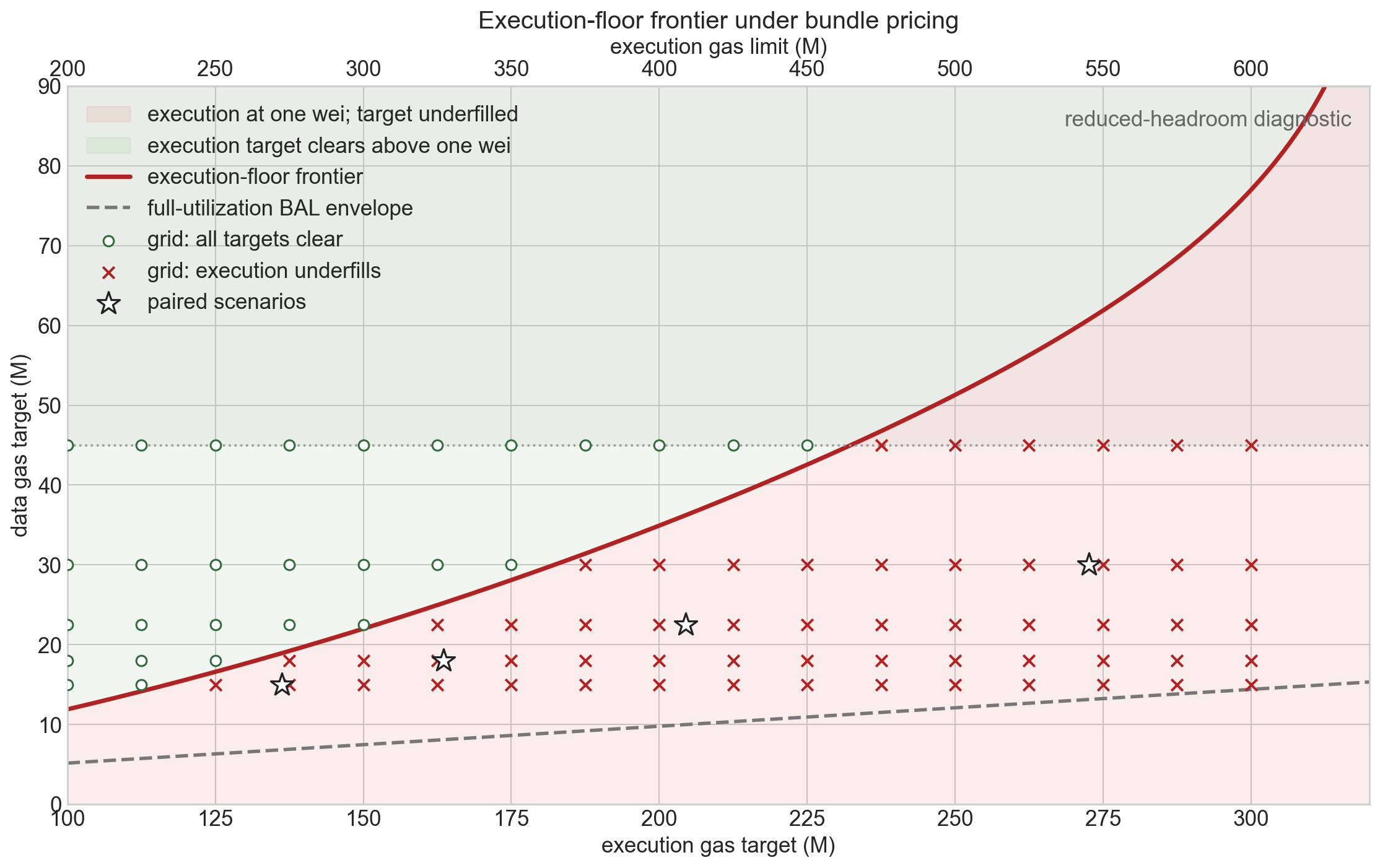
The solid red curve is the exact 1-wei execution-clearing boundary. Green points clear all three targets; red crosses are execution-floor equilibria; stars mark the paired comparability scenarios. The dashed gray line is runtime BAL generated if execution and state both fill their targets. Star signs represent paired scenarios, where we scale the data/execution historical activity proportionally.
The coarse scenario grid crosses five data targets — 15M, 18M, 22.5M, 30M, and 45M — with execution targets from 125M to 300M in 25M steps.
Data and state clear their targets in every cell.
| Data target | Max execution target | Corresponding execution limit | Data fee at boundary (wei / data gas) |
|---|---|---|---|
| 15.0M | 116.9M | 233.7M | 109.0k |
| 18.0M | 131.8M | 263.6M | 40.45k |
| 22.5M | 152.2M | 304.3M | 12.34k |
| 30.0M | 182.2M | 364.5M | 2.764k |
| 45.0M | 232.4M | 464.7M | 353.4 |
From another perspective, execution targets of 125M, 150M, 200M, 250M, and 300M place the 1-wei boundary at data targets of 16.6M, 22.0M, 34.9M, 51.3M, and 77.0M. The 77.0M value is an analytic extrapolation above the displayed 1/2 target ratio.
Full-utilization BAL envelope
At \lambda=0, \rho_A=1 and fixed 75M state gas target, the full-utilization BAL gas scales linearly with the execution gas target in equilibrium:
Above this line, the data target has room for BAL generated at full execution and state utilization. On the line, BAL alone fills the entire data target; below it, BAL at full parent resource utilization exceeds the data target.
A data-market equilibrium base fee can still exist under a data target below this line because a higher data fee reduces BAL-producing activity until total data usage reaches its target. In the scenarios studied, execution then remains below target with its base fee at the one-wei minimum, while data and state clear their targets. In other words, data can clear its target even when execution cannot simultaneously clear its configured target.
The 1-wei execution boundary is stricter than the BAL envelope at any parameter specification tested because positive static-data demand must also fit at a data base fee that leaves room for an execution base fee above 1 wei.
Paired scenarios as comparability benchmarks
The paired scenarios illustrate the floor-bound regime by holding the historical ratio of total counterfactual data gas to metered execution gas constant:
| Execution target | Data target | Regime | Data base fee (wei / data gas) |
Execution target fill | BAL share of data target |
|---|---|---|---|---|---|
| 136.3M | 15.0M | Execution at 1 wei | 109.0k | 85.8% | 39.7% |
| 163.5M | 18.0M | Execution at 1 wei | 40.5k | 80.6% | 36.9% |
| 204.4M | 22.5M | Execution at 1 wei | 12.3k | 74.4% | 33.7% |
| 272.6M | 30.0M | Execution at 1 wei | 2.76k | 66.9% | 29.9% |
We find that all four tested scenarios lie below the execution-clearing boundary, so each settles into an equilibrium in which execution underfills at 1 wei. These scenarios serve solely as comparability benchmarks.
Sensitivity and Robustness
The 1-wei execution boundary is recalculated for all 36 combinations of \lambda\in\{0,0.5,1\}, \rho_A\in\{0.75,1,1.25\}, and the 21-, 35-, 60-, and 75-day elasticity estimates. Each calculation holds the data and state targets fixed, places the execution base fee at 1 wei, and solves for the largest execution target that can still be fully used.
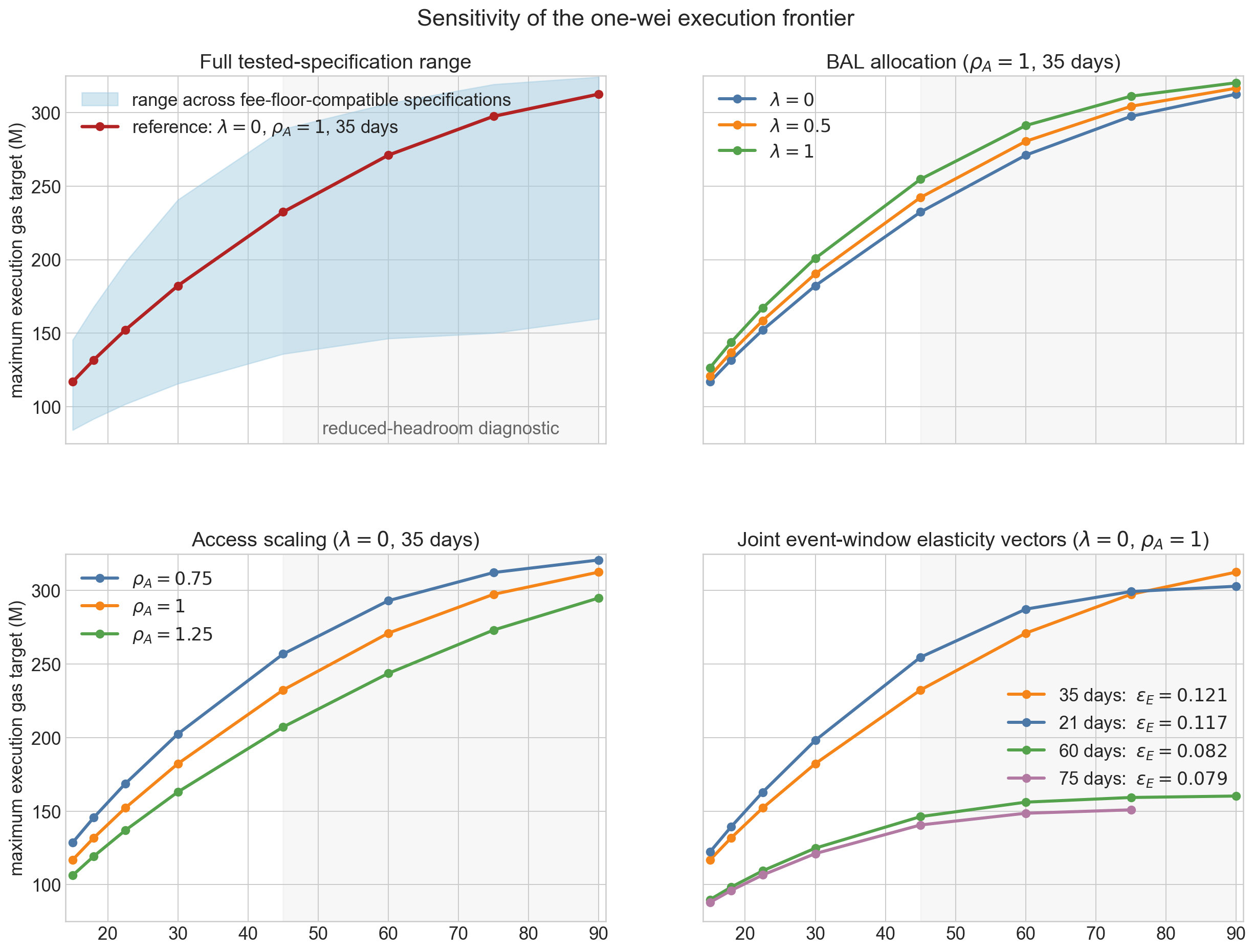
Every one of the 36 specifications has a valid boundary through a 75M data target. At a 90M data target, which equals the data limit, 17 out of 36 specifications would require a data fee below 1 wei, and instead place both base fees at 1 wei with both resources below their targets.
| Data target | Reference maximum execution target boundary | Maximum execution target range across specifications |
|---|---|---|
| 15.0M | 116.9M | 84.2M-145.4M |
| 18.0M | 131.8M | 91.8M-167.8M |
| 22.5M | 152.2M | 101.7M-198.2M |
| 30.0M | 182.2M | 115.7M-240.7M |
| 45.0M | 232.4M | 135.9M-288.8M |
| 60.0M | 271.0M | 146.4M-306.2M |
| 75.0M | 297.4M | 150.1M-319.2M |
| 90.0M (equals the limit) | 312.5M | 159.8M-324.2M |
The directions have a direct interpretation over the studied expansion range. A larger \rho_A generates more execution-linked BAL as execution expands and lowers the supportable execution target. A larger \lambda shifts co-produced BAL toward state activity, which expands less than execution in these scenarios, and therefore raises the boundary.
The elasticity uncertainty under different windows has a larger impact on the execution target boundary than the parameters \lambda or \rho_A. Because state remains interior at its fixed target, \epsilon_{\mathrm{state}} changes only the state fee while the boundary movement comes from \epsilon_{\mathrm{execution}} and \epsilon_{\mathrm{data}}.
Data capacity required for a 300M execution target
Reading the execution-clearing boundary in reverse, we can ask the question: if we want to scale the execution target to 300M, what is the minimum data target required?
First of all, whether the question has an answer at all depends on the demand calibration. Under the 60- and 75-day elasticity vectors, execution demand cannot reach a 300M target at a 1-wei execution fee even if BAL carried no data charge whatsoever. The corresponding execution target ceilings are 160.9M and 152.0M, respectively. The answer below applies to the 21- and 35-day elasticity calibrations.
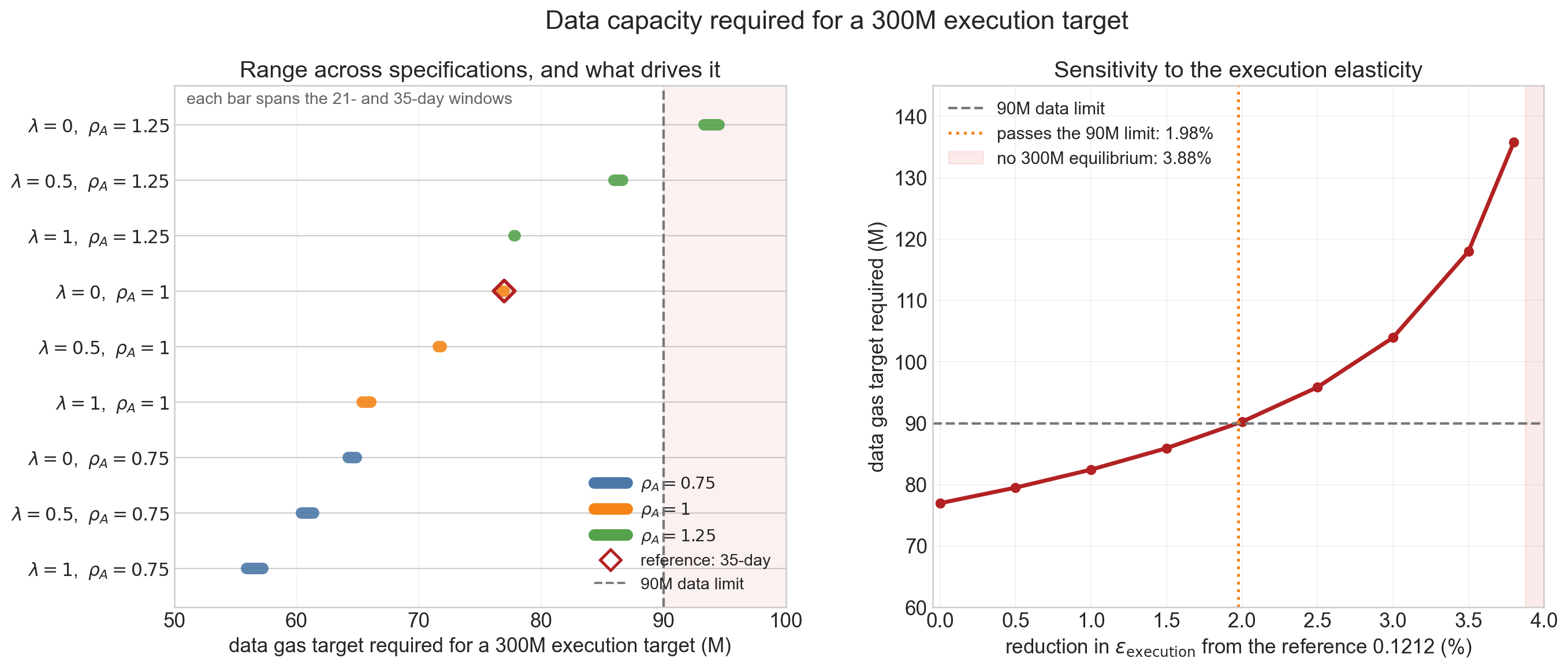
Left: the data target each feasible specification requires for a 300M execution target, sorted. Each bar spans the 21- and 35-day elasticity windows; colour gives \rho_A and the rows within each colour give \lambda. The diamond marks the reference specification and the dashed line the 90M data limit. Right: how the reference requirement responds to a reduction in \epsilon_{\mathrm{execution}} alone, with the limit crossing and the point beyond which no 300M equilibrium exists.
| Elasticity window | Reference \lambda=0, \rho_A=1 | Data target range across \lambda, \rho_A |
|---|---|---|
| 21 days | 76.81M | 57.25M–93.33M |
| 35 days | 76.97M | 55.89M–94.53M |
| 60 days | infeasible | — |
| 75 days | infeasible | — |
Under the reference calibration the answer is approximately 77M. Across the 18 feasible specifications based on the 21- and 35-day elasticity vectors, the minimum data target spans 55.89M to 94.53M:
- the lower bound, 55.89M, comes from \lambda=1 with \rho_A=0.75 on the 35-day vector, where co-produced state access follows state demand and state access scales sub-proportionally with execution.
- the upper bound, 94.53M, comes from \lambda=0 with \rho_A=1.25, also on the 35-day vector, where co-produced state access follows execution demand and state access scales super-proportionally with execution.
A larger \rho_A generates more execution-linked BAL as execution expands, and a smaller \lambda leaves more of the co-produced access on the execution parent, which expands faster than state here; both raise the data target that 300M execution requires.
Relative to the 90M data gas limit:
A 300M execution target consumes 85.5% of the data limit as target, leaving 13.03M of headroom above it. Because the boundary is defined at a 1-wei execution fee, a strictly interior execution fee requires a data target above that value rather than at it.
The comparison with conventional target ratios:
| Data target / target ratio | Largest fully utilized execution target |
|---|---|
| 45M / \frac{1}{2} | 232.4M |
| 60M / \frac{2}{3} | 271.0M |
| 75M / \frac{5}{6} | 297.4M |
| 77M | 300M |
| 90M, the full limit | 312.5M |
How far the boundary moves with the demand elasticities
The reference vector is \epsilon_{\mathrm{execution}}=0.1212, \epsilon_{\mathrm{data}}=0.2295 and \epsilon_{\mathrm{state}}=0.3349, all from the 35-day event windows. Each comparison below perturbs one of them and holds the other two, and every other reference input, fixed.
Execution elasticity.
| Change | \epsilon_{\mathrm{execution}} | Required data target | Movement |
|---|---|---|---|
| -3.0\% | 0.11752 | 103.95M | +35.1\% |
| -2.0\% | 0.11874 | 90.24M | +17.2\% |
| -1.0\% | 0.11995 | 82.44M | +7.1\% |
| -0.5\% | 0.12055 | 79.51M | +3.3\% |
| reference | 0.12116 | 76.97M | — |
| +0.5\% | 0.12177 | 74.74M | -2.9\% |
| +1.0\% | 0.12237 | 72.75M | -5.5\% |
| +2.0\% | 0.12358 | 69.29M | -10.0\% |
| +3.0\% | 0.12479 | 66.35M | -13.8\% |
Three thresholds summarize how reducing \epsilon_{\mathrm{execution}} progressively makes a 300M execution target infeasible:
- 1.98% reduction — data-limit crossing. The required data target exceeds the assumed 90M data limit.
- 3.88% reduction — data-fee floor. Even without the 90M limit, supporting 300M execution would require a data base fee below 1 wei. No all-target-clearing equilibrium therefore exists with both the execution and data base fees bounded below by 1 wei.
- 4.12% reduction — execution-demand ceiling. At this point, 300M execution cannot be supported even if BAL carried no data charge. The 1-wei execution charge alone is already too high.
The response is strongly convex. At the reference point, the local log-elasticity of the required data target with respect to \epsilon_{\mathrm{execution}} is -6.18. This value masks an asymmetry in finite changes: a 1% increase in \epsilon_{\mathrm{execution}} reduces the required data target by 5.5%, whereas a 1% reduction increases it by 7.1%.
The asymmetry becomes more pronounced farther from the reference point. A 0.5% reduction raises the required data target by 3.3%, while a 3% reduction raises it by 35.1%. For capacity design, the feasibility thresholds above are therefore more informative than a single local elasticity.
Data elasticity.
| Change | \epsilon_{\mathrm{data}} | Required data target | Movement |
|---|---|---|---|
| -3.0\% | 0.22259 | 70.94M | -7.8\% |
| -2.0\% | 0.22489 | 72.88M | -5.3\% |
| -1.0\% | 0.22718 | 74.89M | -2.7\% |
| -0.5\% | 0.22833 | 75.92M | -1.4\% |
| reference | 0.22948 | 76.97M | — |
| +0.5\% | 0.23062 | 78.04M | +1.4\% |
| +1.0\% | 0.23177 | 79.12M | +2.8\% |
| +2.0\% | 0.23407 | 81.35M | +5.7\% |
| +3.0\% | 0.23636 | 83.65M | +8.7\% |
Data elasticity moves the frontier in the opposite direction and roughly half as strongly. A 1% increase in \epsilon_{\mathrm{data}} raises the required data target by 2.8%, whereas a 1% increase in \epsilon_{\mathrm{execution}} lowers it by 5.5%. The local log-elasticity with respect to \epsilon_{\mathrm{data}} is $+2.75$, and the response is close to linear over the tested range, so the local value closely matches the finite changes.
The positive sign has a simple explanation. At the frontier, the clearing data fee is below the anchor-equivalent static-data fee, so static-data demand is already expanded relative to its anchor. A larger \epsilon_{\mathrm{data}} makes demand respond more strongly to this lower price, increasing static-data usage and therefore the data target required to support 300M execution.
State elasticity does not move the boundary at all. While state clears its target, q_{\mathrm{state}} is fixed at T_{\mathrm{state}}/m_{\mathrm{state}} whatever its elasticity, so the state-linked BAL it generates is also fixed. State elasticity moves only the state base fee b_{\mathrm{state}}.
Limitations
Isoelastic extrapolation. The calculation carries demand curves far beyond the event windows used to estimate them. Exact wei-level fees and fill rates are conditional functional-form outputs; forecasting future fees would require a dynamic demand and shock model. The regime classification is more stable across the tested assumptions.
Average and marginal BAL intensity. For \rho_A\ne1, the execution parent price uses average BAL intensity, \bar w_{\mathrm{execution}}=w_{\mathrm{execution}}R_{\mathrm{execution}}^{\rho_A-1}. Marginal BAL intensity is \rho_A\bar w_{\mathrm{execution}}. The two coincide at the reference value \rho_A=1; the off-reference cases are reduced-form access-composition sensitivities.
Maintained BAL routing. \lambda determines how co-produced access in state-creating transactions is routed when parent prices move independently. Historical data do not identify this allocation. Values 0, 0.5, and 1 represent maintained structural alternatives.
Takeaways and Next Steps
The execution-clearing boundary is the central result. It traces where, in execution/data target space, the BAL data charge pushes the execution base fee to its 1-wei minimum. In the reference parameterization, a 45M data target places the boundary at a 232.4M execution target. The boundary moves with the structural allocation (\lambda), access-scaling (\rho_A), and elasticity-window assumptions, but retains its qualitative shape across the tested grid. At a 45M data target, the boundary ranges from 135.9M to 288.8M across the tested specifications. The elasticity uncertainty is the largest single source of variation.
A 300M execution target requires a data target of approximately 76.97M, or 85.5% of the fixed 90M limit. Among the feasible specifications under 21- and 35-day elasticity vectors, the requirement ranges from 55.9M to 94.5M. Near the reference point, a 1% reduction in execution elasticity raises the required data target by 7.1%, and a 1.98% reduction moves it beyond the fixed limit. These are therefore conditional capacity benchmarks rather than precise protocol-capacity estimates.
These results provide conditional design guidance for EIP-7999 by identifying the execution/data target combinations that can clear above the 1-wei fee floor. They also establish the equilibrium conditions needed for simulations.