by Fei Wu - This work was partially conducted during my internship at the EF. I thank my mentor @misilva73 for valuable discussions, feedback, and comments.
Overview
In the previous EIP-7999 bundle-priced equilibrium analysis, we identify the execution-clearing boundary — the maximum execution target that can clear before the execution equilibrium base fee reaches 1 wei for a given data target. Building on that equilibrium analysis, this post simulates the EIP-7999 multi-dimensional fee market dynamically by adding block-level demand variation and the fee update rules.
We recover block-level execution, static-data, and state-creation demand shocks, together with a runtime-BAL access-composition shock, from 430,605 consecutive blocks over April and May 2026. We jointly resample the four-dimensional series so that the simulated workloads preserve their temporal dependence and cross-resource co-movement.
We construct a total of 63 EIP-7999 configurations with varied execution gas target from 150M-300M and data gas target from 22.5M-80M. Based on the sampled demand conditions, we simulate each configuration for a one-day burn-in followed by 7 measured days with 50,400 blocks, and repeat the simulation across 32 bootstrap paths. The results describe the long-term dynamics of each EIP-7999 configuration, including how much capacity is utilized, which resource limit binds and how often, and how the base fees move. We show that a configuration that is feasible in equilibrium may perform poorly in the long term when demand varies block by block.
In addition, for each configuration of execution and data gas targets, we simulate varied execution and data gas limits by changing the propagation time relative to the execution time available during a slot. These results reveal resource utilization and the bottleneck resource under different slot-time allocations, thereby informing deadline choices (e.g., attestation and PTC deadlines under ePBS) for scaling under a multi-dimensional fee mechanism.
The results presented in this post can be reproduced from this repository. Throughout this post, we denote by “E300/D80” a configuration with a 300M execution target and a 80M data target. The other configurations are written analogously.
Main results
- Larger execution targets do not always deliver more execution utlization. When a high data fee suppresses BAL-producing activity or the data limit excludes BAL-producing transactions, raising the execution target can increase underutilization.
- The execution base fee is bounded at 1 wei at both low and high data targets for different reasons. A low data target produces a high data fee that prices out BAL-producing execution, whereas a high data target leaves too little hard-limit headroom and excludes BAL-producing execution when the data limit binds.
- Under the fixed 90M data limit and one-half execution target-to-limit ratio, data is the principal bottleneck at high execution targets. Reallocating slot time toward propagation initially increases delivered execution by reducing BAL-related bundle exclusion, even though the execution limit falls. At longer propagation windows, execution becomes the bottleneck.
- The highest delivered execution across all tested scenarios is approximately 270-272.6M gas per block. Under a propagation time \geq 4\text{s}, E300/D80 and E300/D90 deliver approximately 270-272.6M execution gas per block, but these configurations still spend substantial time at hard limits and the 1-wei execution floor.
- Historically anchored lower-pressure configurations delivers 221-223M execution. E225/D52.5 is selected under 3.5-second propagation time, and E225/D60 is selected under 4-second and 4.5-second propagation time. Both deliver 221-223M execution gas on average.
- The attainable execution is highly sensitive to demand uncertainty. Under the 60- and 75-day elasticity calibrations, maximum delivered execution falls to approximately 150M and 142M, respectively.
Notation and central specification
| Group | Notation | Meaning |
|---|---|---|
| Resources | i\in\{\mathrm{execution},\mathrm{data},\mathrm{state}\} | The three separately priced EIP-7999 resources |
| Fees | b_{i,t}, P_{i,t}, p_t, p^0 | Resource base fee, BAL-inclusive effective activity price, and the observed and reference historical effective prices used to recover shocks |
| Capacity | T_i, L_i, h_i | Gas target, hard limit, and normalization denominator; h_i=L_i for execution and data and h_i=T_i for state |
| Block quantities | g_{i,t}^{\mathrm{offered}}, g_{i,t}^{\mathrm{included}} | Gas demanded and gas included in the block after applying the hard limits |
| Demand quantities | q_{i,t}, q_i^0, q_{i,t}^{\mathrm{obs}} | Counterfactual parent activity, historical quantity anchor, and observed historical activity; the data parent quantity is static transaction data before BAL |
| Demand parameters | \widetilde s_{i,t}, s_{i,t}, \epsilon_i, m_i | Raw recovered shock, simulated shock, own-price elasticity, and metering multiplier |
| BAL | \bar w_{\mathrm{execution}}, w_{\mathrm{state}}, \lambda, \rho_A, a_t | Average execution-linked BAL intensity, state-linked BAL intensity, co-produced-BAL allocation, access scaling, and access-intensity shock |
| Outcomes | \bar g_i, U_i | Mean gas usage and target utilization U_i=\bar g_i/T_i |
Unless stated otherwise, the central specification uses the 35-day elasticities (\epsilon_{\mathrm{execution}},\epsilon_{\mathrm{data}},\epsilon_{\mathrm{state}})=(0.121,0.229,0.335), \lambda=0, \rho_A=1, and a 75M state target. The initial target-grid experiment uses a 90M data limit and an execution target-to-limit ratio of 1/2. We also note that due to a recent change in EIP-8038, the execution multiplier changes from 1.5379 to 1.448. We use the updated value 1.448 throughout this analysis.
Dynamic simulation framework
We simulate the bundle-priced EIP-7999 mechanism described in the previous equilibrium analysis. Execution, data, and state each have their own base fee and EIP-4844-style fake-exponential update rule. A transaction’s execution and state creation activity also generate EIP-8279 runtime BAL bytes that consume data gas, so users respond to BAL-inclusive parent prices:
Importantly, when the data limit binds, the bundle inclusion rule removes the parent execution/state-creation transaction together with its generated BAL. The update rules then update the base fee based on included gas in the block.
EIP-7999 fee update rules. EIP-7999 accumulates a normalized excess-gas counter for each resource and exponentiates it. Away from integer rounding, the resulting fee movement is approximately
where h_i denotes the normalization denominator. As in the updated EIP-7999 spec, h_i=L_i for execution and data, while h_i=T_i for state because state has no hard limit. Above-target usage raises the base fee, while below-target usage lowers the base fee, subject to the 1-wei minimum.
Recovering empirical demand shocks
To simulate the fee mechanism, we need a block-by-block demand path to answer how long congestion lasts, how extreme a burst becomes, or how quickly a fee recovers. Repeating average demand can test equilibrium convergence but cannot reveal dynamic outcomes. We therefore recover the demand variation embedded in historical blocks and use it to construct counterfactual shock paths.
We consider three demand shocks and one access-composition shock because EIP-7999 has three priced resources but four economically distinct sources of block-level variation. Execution, static transaction content data, and state each have an independently modeled demand curve, so each requires a shock that shifts how much of that activity users want at a given price.
Parent execution and state activities do not determine BAL exactly because the transaction mix changes across blocks. Two blocks can contain the same total execution and state creation activity while producing different BAL: one may be compute-heavy, while the other repeatedly accesses accounts and storage. The fourth shock, a_t, captures this conditional access intensity. It scales the BAL generated per unit of parent execution, while the three parent demand curves remain the behavioral source of BAL demand.
The four shocks and their historical inputs are:
| Shock | Historical input | Role in the simulation |
|---|---|---|
| s_{\mathrm{execution},t} | observed execution activity | shifts the execution demand curve |
| s_{\mathrm{data},t} | observed static transaction-data activity | shifts demand for calldata and other static data |
| s_{\mathrm{state},t} | observed state creation | shifts the state-creation demand curve |
| a_t | runtime BAL relative to BAL predicted by parent activity | changes the access intensity of the transaction mix |
Removing the historical price response
Observed activity in historical blocks does not directly reflect the exogenous demand shock. A block can contain unusually high activity because the historical base fee was low, because underlying willingness to transact was high, or because both occurred at the same time. Replaying observed quantities directly would retain the historical price response and then apply another price response under the counterfactual fee mechanism.
Therefore, we first remove the response attributed to the historical base fee. For execution, static data, and state creation, let q_{i,t}^{\mathrm{obs}} be observed block activity, q_i^0 its historical mean per block, p_t the historical shared base fee, p^0 the reference fee, and \epsilon_i its estimated elasticity. The maintained demand equation is
so the price-adjusted demand condition is
The recovered \widetilde s_{i,t} measures how high or low activity was relative to what the maintained demand curve predicts at that block’s fee. For example, suppose execution activity is 20% above its historical mean while the fee is twice its reference value. With \epsilon_{\mathrm{execution}}=0.121, \widetilde s_{\mathrm{execution},t}=1.20\times2^{0.121}\approx1.30. Observed execution is only 20% above its mean, but the recovered demand condition is approximately 30% above normal because the high historical fee was already suppressing activity.
Runtime BAL is handled differently because users do not independently demand BAL bytes. Based on the previous analysis, we first predict BAL from the observed parent activity:
The raw access-intensity ratio is observed runtime BAL relative to this prediction:
Thus, \widetilde a_t=1.2 means that the block produces 20% more runtime BAL than predicted from its execution and state activity. We then normalize a_t so that applying it to the predicted BAL preserves average historical BAL. Blocks predicted to carry more BAL receive more weight because the same percentage increase represents more data gas in those blocks. For example, a 10% increase in a block with 10M predicted BAL gas changes total BAL ten times as much as a 10% increase in a block with 1M. The adjustment retains the timing of unusually high and low access intensity while keeping average BAL equal to its historical anchor. Together, the three price-adjusted parent shocks and the access-intensity shock form the vector \mathbf s_t=(s_{\mathrm{execution},t},s_{\mathrm{data},t},s_{\mathrm{state},t},a_t) used in the replay.
Constructing simulated demand paths
The empirical panel contains 60 days from 2 April through 31 May 2026, covering 430,605 consecutive blocks. We collect block-level execution, static data, state creation, and historical fees from Xatu tables and reconstruct the EIP-8279 runtime BAL meter for these blocks.
The simulation receives one four-dimensional shock vector for every block, containing execution, static-data, state, and access-intensity conditions. Synthetic paths are constructed to preserve historical persistence, clustered bursts, recurring demand patterns, and cross-resource co-movement. Contiguous 3,200-block historical segments, approximately 10.7 hours each, preserve the ordering and joint movement of the shocks within each segment. Each path is normalized around the historical mean quantities so that resampling changes the timing and clustering of demand without shifting its anchor.
Each simulated path contains 7,200 burn-in blocks, which ensures the fee market starts around the resources’ equilibrium base fees, followed by 50,400 measured blocks (i.e., equivalent to 7 days). We generate 32 paths and give every configuration the same sampled demand conditions, so differences across mechanisms and capacity settings are paired comparisons rather than differences in sampled workloads.
At each simulated block, the current effective prices determine movement along the demand curves while the sampled shocks shift those curves:
Runtime BAL is generated after the parent execution/state quantities are realized. The figure below shows the gas usage and fees of each resource dimension in one example simulation path of the E225/D60 configuration, with 75M state target, 90M data limit, and 1/2 execution target-to-limit ratio.
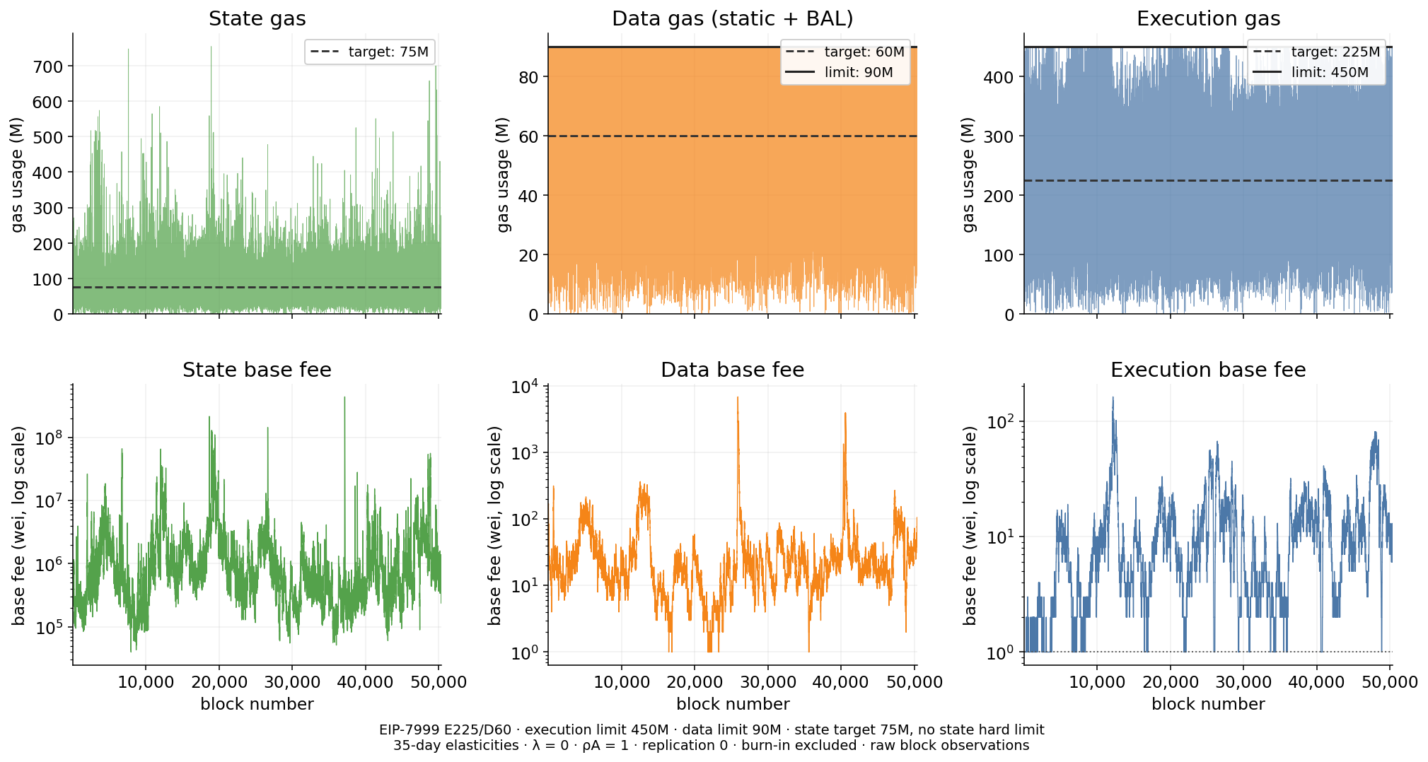
Block-level gas usage and base fees for E225/D60 over 50,400 simulated blocks. The upper panels show state, data—including static content and BAL—and execution gas usage. Dashed lines mark targets of 75M, 60M, and 225M. Solid lines mark the 90M data limit and 450M execution limit. State has no hard limit. The lower panels show the corresponding base fees in wei on logarithmic scales. The simulation uses the 35-day elasticity vector, \lambda=0, and \rho_A=1.
Outcome metrics
| Metric | Interpretation |
|---|---|
| Delivered execution | Mean included execution gas across measured blocks and bootstrap paths |
| Execution target utilization | Delivered execution divided by the configured execution target |
| Full block fraction | Fraction of blocks whose included execution or data gas equals the hard limit |
| Execution fee bounded at 1 wei | Fraction of blocks with a 1-wei execution fee while included execution gas remains below target |
| Mean absolute target deviation | \operatorname{mean}\left[\frac{|g_{i,t}-T_i|}{T_i}\right] |
| Price variation | Standard deviation of block-to-block log changes in each resource’s effective activity price, \operatorname{sd}(\Delta\log P_i). |
We note that the 1-wei metric distinguishes a fee that merely touches 1 wei from the update rule that would reduce the fee further if the protocol allowed it.
Target Grid Under a Fixed 90M Data Limit and 1/2 Execution Target-to-Limit Ratio
The initial target-grid experiment is designed to isolate the interaction between execution and data targets. We hold the execution target-to-limit ratio fixed at T_{\mathrm{execution}}/L_{\mathrm{execution}}=1/2. This gives each execution target the same relative burst headroom and the same normalized fee-update response. The data limit is fixed at 90M, while the execution limit scales with its target. The experiment covers seven execution targets from 150M to 300M and nine data targets from 22.5M to 80M, producing 63 configurations. We simulate all 63 configurations and examine their execution support, limit pressure, and price variation.
Execution support and 1-wei floor operation
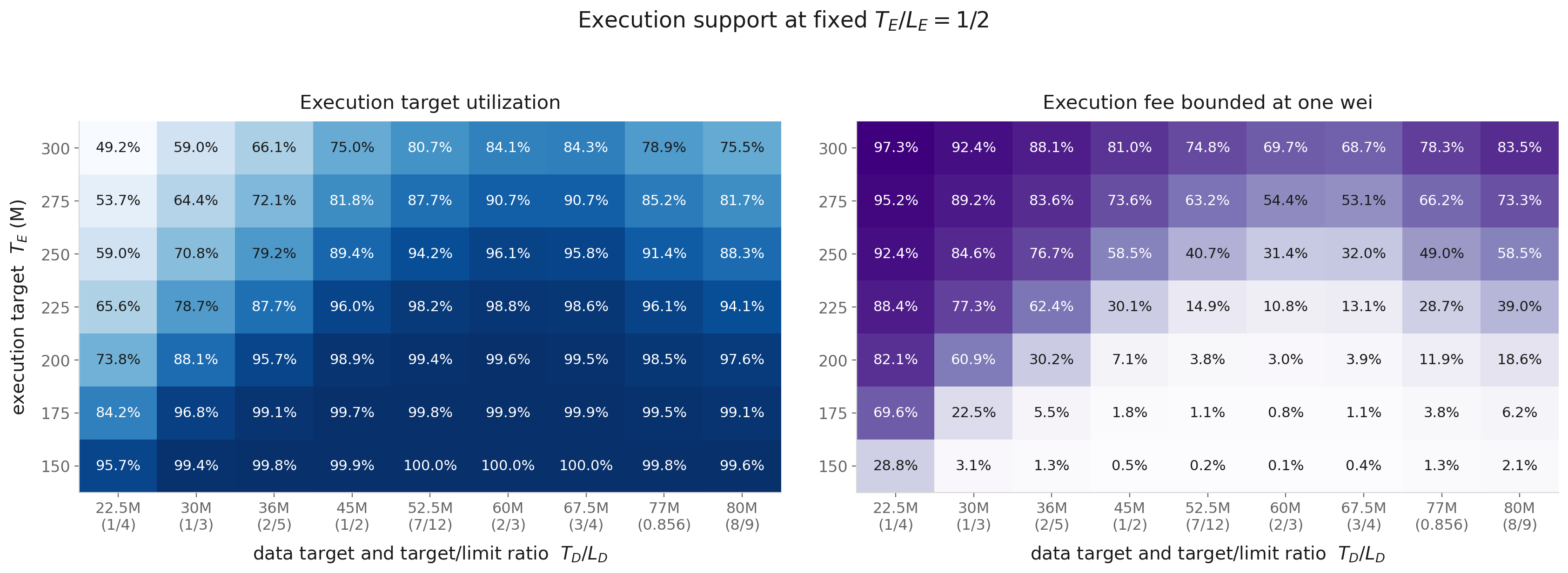
Left: Execution target utilization: delivered execution gas as a fraction of the execution target. Right: the fraction of blocks in which the execution fee is bounded at 1 wei. Each cell is the mean across 32 bootstrap paths.
We observe that, at each execution gas target, as the data gas target increases, the delivered execution gas (execution target utilization) is low at first, then increases with the data gas target, and eventually drops when data target is high and close to its 90M limit. Correspondingly, when execution target utilization is low, the execution base fee is more often bounded at the 1-wei minimum. The execution gas underfills its target, while the protocol cannot further reduce its base fee to be lower than 1 wei. This “U-shape” effect is especially significant when the execution gas target is high.
The two sides of the “U-shape” effect have different causes.
At low data targets, execution is constrained by data price. A low target requires a high data fee to contract static-data demand. The same data fee prices the BAL generated by parent execution, so the execution dimension reduces its fee until it reaches 1 wei. However, the 1-wei fee still cannot attract enough demand to fill the execution target because the BAL-inclusive bundle price is expensive, especially under high execution targets, contributing to low target utilization and fee being bounded at 1 wei in most blocks.
At high data targets, execution is constrained by data limit. A high data target and low data fee expands static data demand, while leaves small headroom beneath the 90M data limit. When a positive data demand shock occurs and demanded data gas exceeds the 90M limit, additional BAL cannot be included in the block, causing the associated execution to be excluded from the block. At E300/D80, demanded data gas averages 119.5M and the data limit is reached in 59.2% of the blocks. Therefore, execution target underfills even while execution-limit capacity remains available, thus the fee is bounded at 1 wei in most blocks.
The static equilibrium boundary we derived for 300M execution target in the previous analysis is insufficient to reflect long-term dynamics. E300/D77 lies close to the 1-wei equilibrium frontier. However, due to the data limit constraint, it delivers only 226.4M execution gas, or 75.5% of its target, with the execution base fee being bounded at 1 wei in 83.5% of blocks.
Data-limit pressure and composition
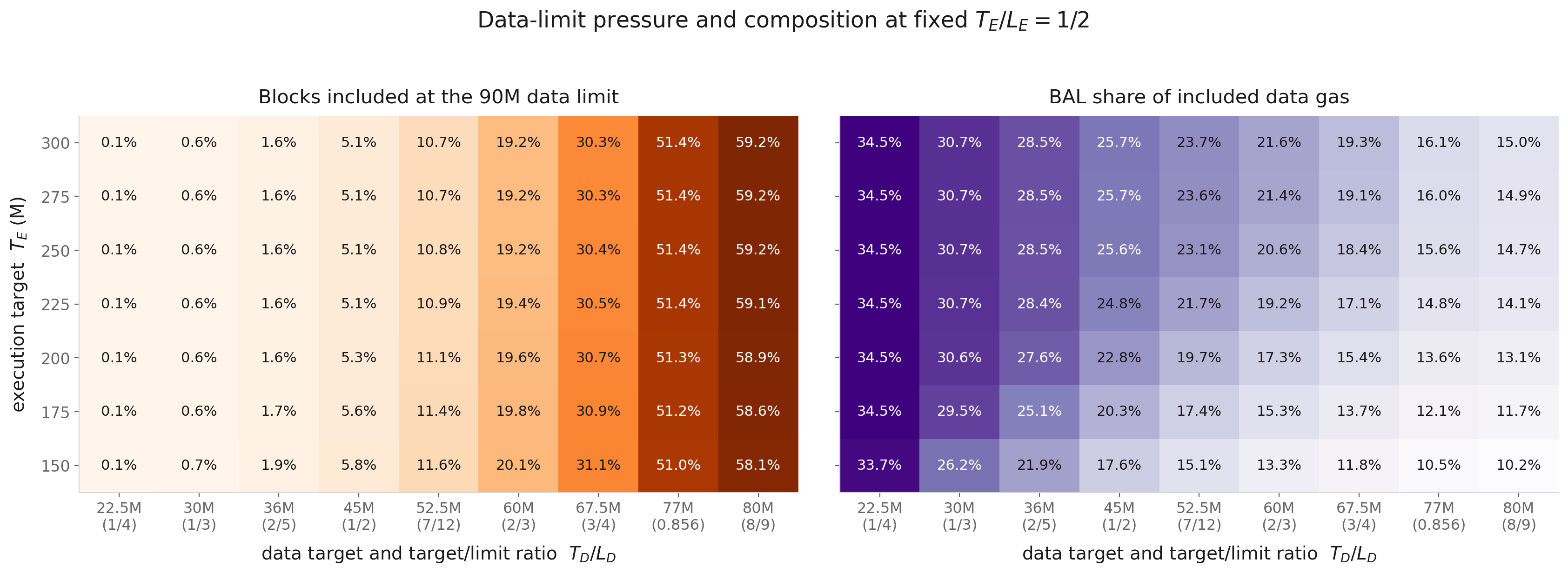
Left: the fraction of blocks whose included data gas equals the 90M limit. Right: BAL as a share of included data gas.
The data target ratio is the dominant congestion lever. At a 1/2 data target ratio, blocks included at the data limit remain close to 5% across execution targets from 150M to 300M. At a 8/9 target ratio, the same frequency is approximately 59% throughout the grid. The cause is intuitive: at 80M target under a 90M limit, only 10M of headroom remains. Ordinary positive demand shocks can fill the remaining space very quickly.
Higher execution targets change the data mix. At a fixed data target, raising the execution target lowers the execution fee and expands execution activity. This produces more execution-linked BAL. Since total data demand still has to clear around the same data target, the data fee adjusts upward and contracts static-data demand. The composition of included data consequently shifts from static transaction data toward BAL.
This composition shift explains the small decline in data-limit frequency as the execution target rises at a fixed data target ratio. The static-data shock is more dispersed than the execution shock in the empirical panel. Execution-linked BAL inherits much of its variation from execution activity, while the conditional access-intensity shock is narrower and mildly negatively correlated with execution. Replacing a small amount of independently volatile static-data demand with execution-linked BAL therefore slightly reduces the extremity of the upper tail of total data demand.
Execution and data price variation
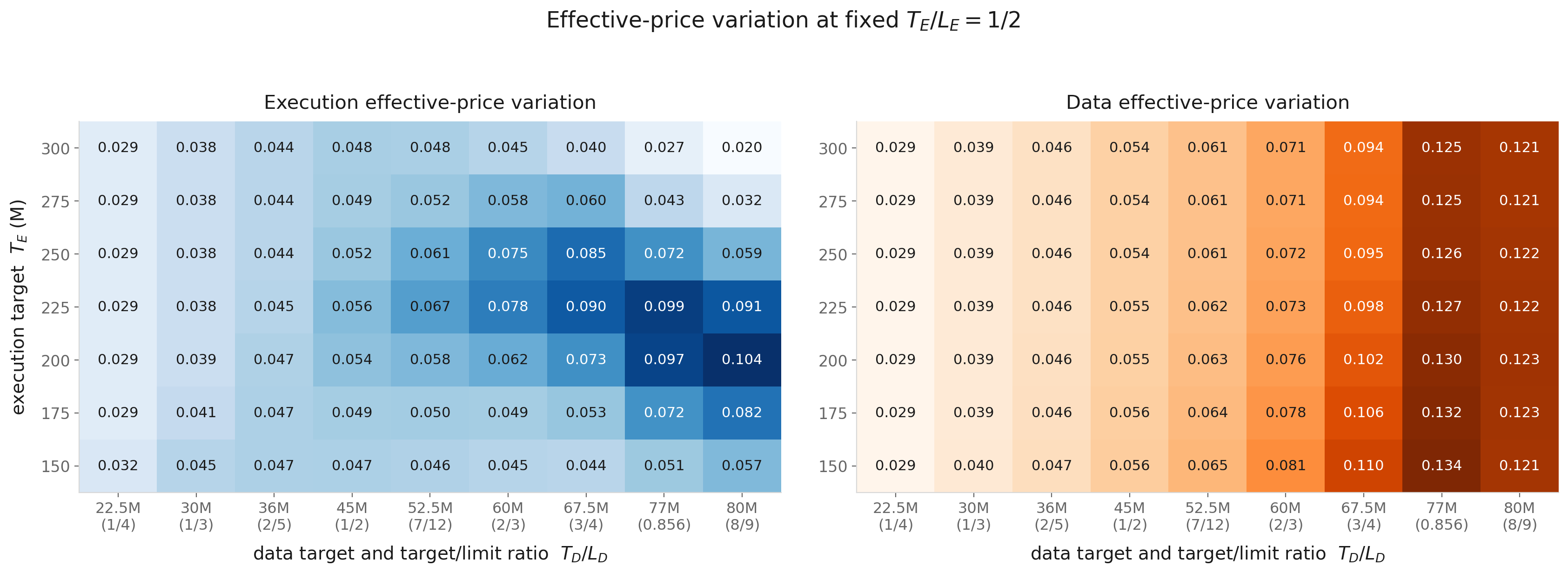
Standard deviation of block-to-block log changes in the execution and data effective activity prices.
Execution-price variation is non-monotonic. It is relatively low in regions where the execution base fee is often bounded at 1 wei. At low data targets, this happens because the high BAL data charge suppresses execution demand. At high data targets and large execution targets, it happens because data-limit exclusion repeatedly removes BAL-producing execution and the execution base fee can no longer be adjusted downward from 1 wei.
This explains why low measured execution-price variation may not be desirable, because the low variation is primarily caused by floor compression not stable market clearing. At E300/D80, execution-price variation is only 0.02, but the execution fee is bounded at 1 wei in 83.5% of blocks and execution delivers only 75.5% of target.
The largest execution-price movements tend to occur in the transition region, where the execution fee sometimes reaches the 1-wei floor but still spends substantial time above it. There, both the execution base fee and the BAL data charge remain active sources of price movement.
Data-price variation generally rises with the data target ratio and changes little with the execution target. The data controller divides the included-gas gap by the fixed 90M limit, so the same proportional demand swing produces a larger absolute gas gap at a larger target. Along the E300 row, data-price variation rises from 0.029 at D22.5 to 0.125 at D77, before falling slightly to 0.121 at D80 as persistent clipping compresses the response.
At D80, the target lies only 10M below the fixed 90M limit. More demanded data gas are clipped to exactly 90M, making shocks above the limit indistinguishable. In addition, data base fee reaches the 1-wei minimum more frequently, making more downward updates bounded at 1 wei and producing zero price changes. These boundary effects reduce measured price variation slightly, even as congestion increases.
Summary
We here summarize the metrics of a few representative configurations.
| Setting | Data target ratio | Delivered execution (target utilization%) | Full on data | Execution fee bounded at 1 wei | Execution-price variation | Data-price variation | State-price variation |
|---|---|---|---|---|---|---|---|
| E200/D45 | 1/2 | 197.8M (98.9%) | 5.3% | 7.1% | 0.054 | 0.055 | 0.150 |
| E225/D52.5 | 7/12 | 220.9M (98.2%) | 10.9% | 14.9% | 0.067 | 0.062 | 0.149 |
| E250/D60 | 2/3 | 240.3M (96.1%) | 19.2% | 31.4% | 0.075 | 0.072 | 0.149 |
| E275/D67.5 | 3/4 | 249.4M (90.7%) | 30.3% | 53.1% | 0.060 | 0.094 | 0.148 |
| E300/D77 | 0.856 | 236.6M (78.9%) | 51.4% | 78.3% | 0.027 | 0.125 | 0.149 |
From this table, we can see why an E300/D77 configuration may not be ideal in practice despite feasible in equilibrium. On average, it delivers only 236.6M execution gas, or 78.9% target utilization, but contributes to more than half of blocks being full and execution fee being bounded by 1 wei at 78.3% of blocks.
We also observe that price variation of state is much higher than execution and data. This is because a block does not have a gas limit for state, and the state excess gas is normalized by its target when updating the fee, which means the same proportional target deviation produces twice the execution fee response when execution’s target-to-limit ratio is 1/2.
Changing slot-time allocation and target-to-limit ratios
The preceding execution-data target grid analysis use a fixed 90M data gas limit, which is informed by propagation model with a 3-second window under the current ePBS slot-time allocation. Configurations like E300/D77 and E300/D80 are constrained by the 90M data gas limit. One way to support larger blocks is to move the ePBS PTC payload deadline later into the slot. This allows more propagation time and a higher data gas limit, at the cost of less execution time and lower execution gas limit. In other words, given a combination of execution and data gas targets, changing the propagation time reduces the data target-to-limit ratio and increases the execution target-to-limit ratio.
We next replace the normalized 1/2 execution-limit convention with physical execution and data limits derived from the propagation/execution time allocations. We change the propagation time while holding the slot budget of propagation plus execution fixed at 9 seconds (i.e., the attestation deadline is fixed at t=3 seconds) to study different combinations of data and execution limits:
where v_{\mathrm{execution}}=100\mathrm{M} gas per second. The empirical propagation fit is
The corresponding data and execution gas limits under different slot-time allocations are:
| Propagation time | Execution time | Data limit | Execution limit |
|---|---|---|---|
| 3.0s | 6.0s | 90M | 600M |
| 3.5s | 5.5s | 108.4M | 550M |
| 4.0s | 5.0s | 126.9M | 500M |
| 4.5s | 4.5s | 145.4M | 450M |
| 5.0s | 4.0s | 163.9M | 400M |
We then run simulations for all 63 configurations in the execution-data target grid under different slot-time allocations, varying execution and data limits (in other words, the target-to-limit ratios). In addition, we consider larger data targets, such as 90M and 100M, which are enabled under longer propagation time windows.
For simplicity and clarity, we present the metrics of configuration E300/D80 under different slot-time allocations. E300/D80 provides a good example: Under the normal 3-second propagation time, E300/D80 is constrained by the 90M data limit, and delivers low execution target utilization and high fee floor-bounded frequency.
The table and figure below show how the metrics of E300/D80 change with longer propagation time:
| Propagation time | Execution limit | Data limit | Mean data fee | Demanded data gas | Delivered execution / utilization | Full on data | Full on execution | Execution fee bounded at 1 wei |
|---|---|---|---|---|---|---|---|---|
| 3.0s | 600M | 90M | 5.05 wei | 119.5M | 226.4M / 75.5% | 59.2% | 0.1% | 83.5% |
| 3.5s | 550M | 108.4M | 18.53 wei | 95.6M | 261.9M / 87.3% | 28.4% | 0.6% | 62.0% |
| 4.0s | 500M | 126.9M | 44.46 wei | 87.9M | 270.7M / 90.2% | 15.5% | 2.3% | 56.2% |
| 4.5s | 450M | 145.4M | 56.76 wei | 84.8M | 271.9M / 90.6% | 8.6% | 6.9% | 55.9% |
| 5.0s | 400M | 163.9M | 61.03 wei | 83.5M | 268.5M / 89.5% | 5.0% | 13.8% | 58.1% |
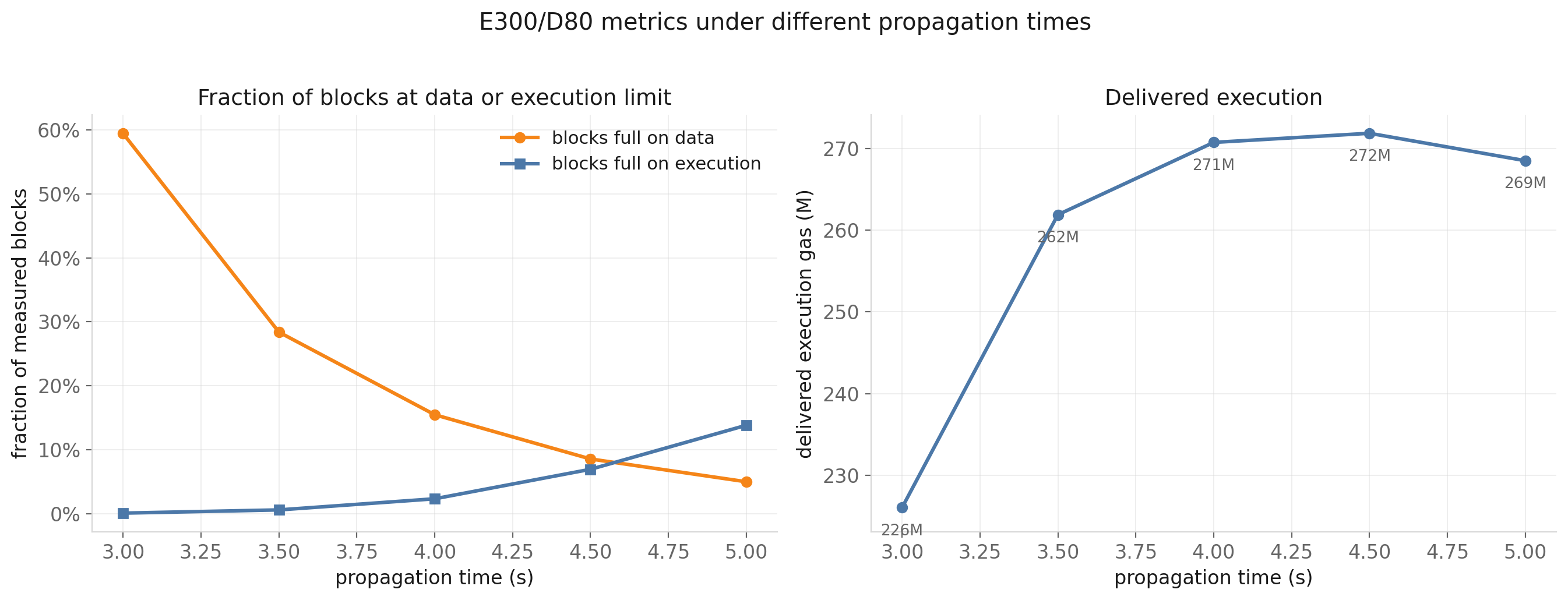
We observe that increasing the propagation time from 3 seconds to 3.5 seconds or 4 seconds substantially relieves the data limit pressure and delivers more execution gas because execution-generated BAL is less often constrained by the data limit. However, due to the execution fee being floor-bounded in nearly half of the blocks, average delivered execution gas still cannot reach the 300M target.
The additional data capacity does not merely include more of the original 119.5M demanded data gas. It changes the fee equilibrium: the fee mechanism prices offered demand downward while allowing more parent execution to be included. At 3 seconds, the 90M data limit leaves only 10M above the 80M target, keeping the mean data fee at 5.05 wei. Raising the data limit to 126.9M exposes more demand above the target to the fee mechanism and raises the mean data fee to 44.46 wei. Static-data demand consequently contracts from 103.6M to 73.1M, bringing total demanded data down from 119.5M to 87.9M even though mean included data remains close to the 80M target. The higher data fee also reduces offered execution from 308.6M to 290.5M through the BAL-inclusive execution price. Even so, the larger data limit admits more BAL-generating execution, raising delivered execution from 226.4M to 270.7M.
At propagation times of 4.5 seconds and longer, we observe that execution starts to be the bottleneck and more blocks hit the execution limit under shorter execution times. Therefore, execution utilization drops although the block is no longer constrained by the data limit.
An important caveat is that, although longer propagation times such as 4.5 seconds and 5 seconds support a larger data gas limit, the corresponding payload size (approximately 9 MiB for 145.4M data gas and over 10 MiB for 163.9M data gas) may not be feasible for the network at the p2p layer. We include these configurations in this analysis as a theoretical exploration.
Candidate Configurations
After exploring EIP-7999 configurations with execution and data targets ranging, we introduce two standards to select an candidate configuration under different propagation times.
Maximum-throughput
| Propagation | Configuration | Equilibrium execution fee | Delivered execution | Execution fee bounded at 1 wei | Full on execution | Full on data |
|---|---|---|---|---|---|---|
| 3.0s | E300/D67.5 | 1 wei (bounded) | 252.929M | 68.73% | 0.24% | 30.44% |
| 3.5s | E300/D77 | 1 wei (bounded) | 263.798M | 60.95% | 0.66% | 24.63% |
| 4.0s | E300/D80 | 1 wei (bounded) | 270.741M | 56.15% | 2.32% | 15.47% |
| 4.5s | E300/D90 | 1 wei (bounded) | 272.598M | 54.29% | 5.38% | 14.14% |
| 5.0s | E300/D90 | 1 wei (bounded) | 271.036M | 55.60% | 13.27% | 8.40% |
We list the configuration that delivers the most execution gas usage on average across all 32 simulation bootstraps. We note that in some bootstraps, other configurations can deliver more execution than the listed ones.
Selecting the configuration with highest mean delivered execution has clear scaling benefits. However, there are obvious tradeoffs: the fee mechanism cannot adjust the execution base fee downward in 54.3%–68.7% blocks because it is bounded by 1 wei, and 17.8%–30.7% blocks are hitting either the execution or data gas limit.
Historically anchored capacity-pressure rule
To allow the fee mechanism to adjust downward and control the full block rate within an acceptable range, we first filter the configuration whose equilibrium execution base fee is strictly higher than 1 wei, and full block rate within a range derived from historical data with some tolerance. We then select the configuration that delivers the maximum execution among them. In addition, we also bound execution gas usage deviation from the target, similarly as we do for full block rate.
Across 860,505 canonical blocks from February through May 2026, 4.73% of blocks reach at least 98% of the gas limit and the mean absolute distance from the gas target is 35.35%. We allow a 20% tolerance around both values, giving ceilings of 5.68% for near-limit frequency and 42.42% for execution target deviation.
| Propagation | Configuration | Equilibrium execution fee | Delivered execution | Execution deviation | Blocks near either limit |
|---|---|---|---|---|---|
| 3.0s | E175/D36 | 69.511 wei | 173.644M | 32.02% | 1.92% |
| 3.5s | E225/D52.5 | 7.135 wei | 221.415M | 31.63% | 5.21% |
| 4.0s | E225/D60 | 11.014 wei | 223.004M | 31.54% | 5.34% |
| 4.5s | E225/D60 | 11.014 wei | 222.966M | 31.51% | 5.16% |
| 5.0s | E200/D67.5 | 36.848 wei | 199.674M | 31.41% | 5.45% |
E225/D60 delivers approximately 223M execution gas under 4-second and 4.5-second propagation times.
Parameter sensitivity
The central results use the 35-day elasticity vector, \lambda=0, and \rho_A=1. The sensitivity analysis replays all combinations of the four elasticity windows, BAL routing \lambda\in\{0,0.5,1\}, and access-scaling intensity \rho_A\in\{0.75,1,1.25\} at every slot-time allocation. It then reruns the complete execution-data target grid under the same shock paths, allowing the maximum-throughput and balanced configurations to be selected again.
Similarly, for simplicity and clarity, we show how delivered execution and full block rate of configuration E300/D80 change with parameter specifications.
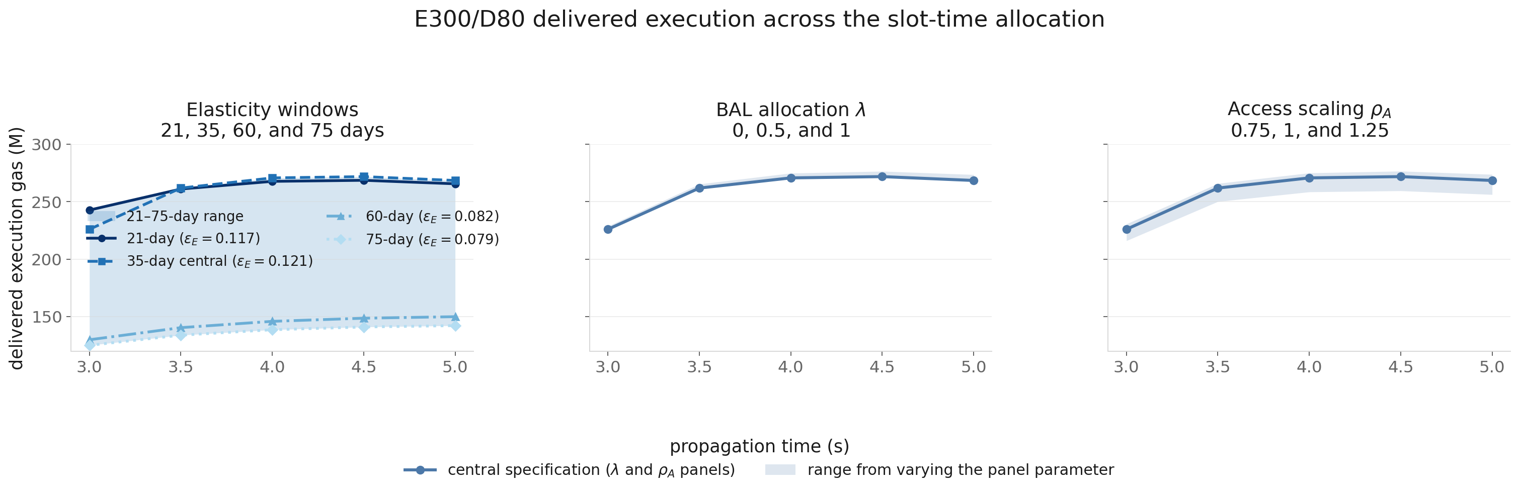
Delivered execution under fixed E300/D80 targets. In the elasticity panel, the legend reports the execution elasticity associated with each estimation window. Colour, line style, and marker identify the four windows, while the shaded region spans their full range. The remaining panels vary \lambda or \rho_A around the central specification.
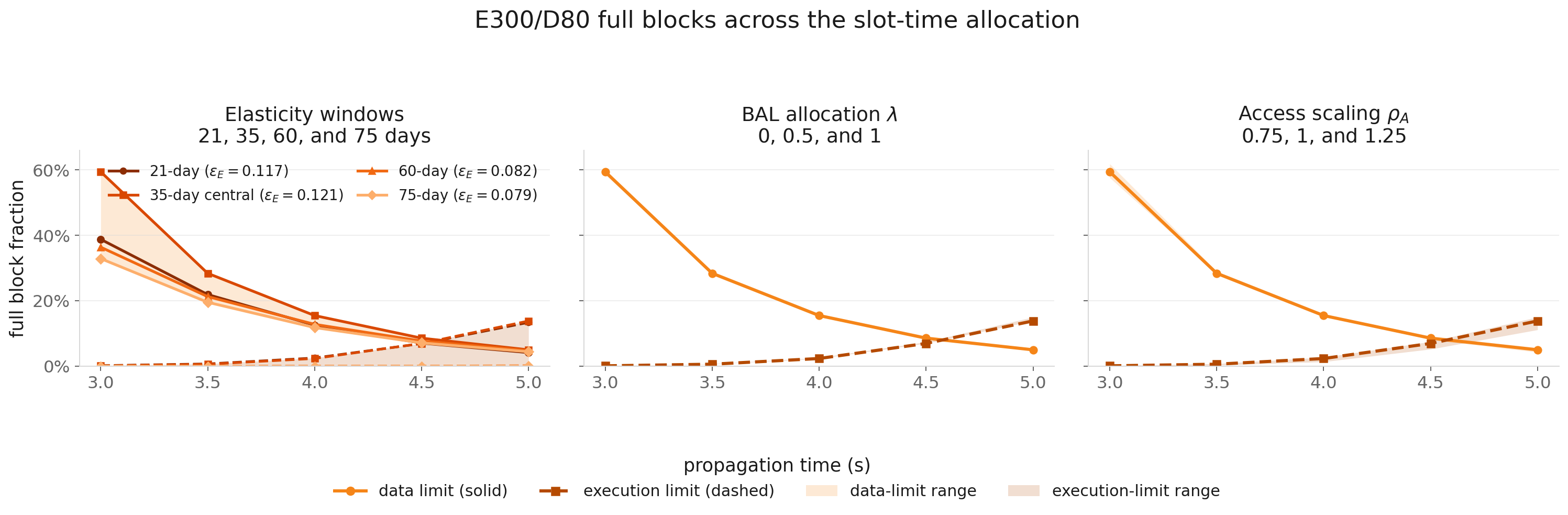
Full data and execution block rate under fixed E300/D80 targets. Colour and marker identify the elasticity window, solid lines report the data limit, and dashed lines report the execution limit. Each shaded region shows the range obtained by varying the parameter named in that panel while holding the other parameters at their central values.
The BAL routing parameter \lambda has the smallest effect: at fixed E300/D80 it moves delivered execution by no more than 5.1M across the tested scenarios. Changing the access-scaling parameter \rho_A produces a 14.6M–17.5M range. The elasticity window dominates the sensitivity because the 60- and 75-day execution elasticities are too low for current modeled demand to support a 300M target even at the 1-wei minimum. Their delivered execution rises modestly with propagation time because the larger data limit constrain execution through BAL less often, but it remains near the 1-wei demand ceilings of approximately 152M and 144M rather than approaching the 300M target.
Nevertheless, the patterns we observe hold under different parameter specifications: as the propagation time and data gas limit increase, the mechanism delivers more execution gas usage until execution becomes constrained by the shorter execution window and lower execution limit. The patterns hold analogously for other configurations.
Robustness of the candidate selections
To see how parameter specifications affect configuration candicate selection, we present the selected candidate under the central specification and seven alternatives: the other three elasticity windows, two other \lambda values, and two other \rho_A values. Each alternative changes one parameter while the others remain central. Within each specification, we select once across all propagation times and target pairs.
| Maintained specification | Maximum-throughput candidate | Historically anchored low-pressure candidate |
|---|---|---|
| 35-day elasticities, \lambda=0, \rho_A=1 (central) | 4.5s, E300/D90, 272.6M | 4.0s, E225/D60, 223.0M |
| 21-day elasticities | 4.5s, E300/D80, 268.7M | 4.0s, E250/D52.5, 242.5M |
| 60-day elasticities | 5.0s, E300/D80, 150.0M | 5.0s, E150/D80, 142.3M |
| 75-day elasticities | 5.0s, E300/D80, 142.2M | — |
| \lambda=0.5 | 4.5s, E300/D80, 274.3M | 4.0s, E225/D60, 223.5M |
| \lambda=1 | 4.5s, E300/D80, 276.5M | 4.0s, E250/D52.5, 243.6M |
| \rho_A=0.75 | 4.5s, E300/D80, 276.6M | 4.0s, E250/D52.5, 243.6M |
| \rho_A=1.25 | 5.0s, E300/D100, 265.7M | 4.0s, E225/D60, 220.2M |
Among the demand-feasible specifications—the central and 21-day elasticity calibrations together with the \lambda and \rho_A variations—the maximum-throughput candidate is highly stable at the level of the slot-time allocation. Nearly every specification selects 4.5 seconds of propagation, an execution target of 300M, and a data target between 80M and 90M. The super-proportional access specification \rho_A=1.25 selects 5 propagation time and 100M data limit, due to the BAL pressure it faces. Delivered execution ranges from 265.7M to 276.6M.
The historically anchored low-pressure selection is stable under demand-feasible specifications — E250/D52.5 at either 3.5 or 4.0 seconds of propagation time, where data and execution physical constraints are better balanced. The super-proportional access case \rho_A=1.25 instead selects E225/D60.
The 60- and 75-day elasticity calibrations form a different regime. Their modeled execution demand reaches its 1-wei ceiling near 152M and 144M, so no slot-time allocation can make a 300M target attainable. The 60-day calibration selects a 5.0-second historically anchored design delivering 142.3M, while no configuration under the 75-day calibration passes the historically anchored rule. We report these calibrations as uncertainty about demand support.
Overall, the bottleneck-handover result is more robust than the exact candidate cell. BAL routing \lambda has little effect on the selected region, while access-scaling \rho_A can shift the preferred execution/data target. The elasticity calibration determines whether the high-throughput region is economically reachable at all.
Limitations
Demand and BAL extrapolation. The elasticity estimates, access-scaling parameter, and BAL attribution are transported beyond their historical calibration ranges. Target configurations tested above require activity several times above the historical anchor and operate near the 1-wei fee minimum. Theses results conditional on the maintained isoelastic and BAL-scaling assumptions.
Physical capacity mapping. The slot-time allocation results depend on the assumed propagation model, 100M-gas-per-second execution rate, and the ePBS PTC specifications. Runtime-metered BAL and final encoded BAL are also different physical objects. The reported limit pairs are conditional capacity scenarios rather than network-safety recommendations.
Aggregate block-level inclusion and no backlog. The simulator removes BAL and the parent execution or state activity proportionally when the data hard limit binds, rather than selecting individual transactions. It also treats demand excluded from one block as unserved flow, rather than returning the transactions to the mempool to be considered in later blocks.
Conclusion
The dynamic simulation changes how the static execution-clearing boundary should be interpreted. A target combination can clear under mean demand yet operate poorly block by block. With a low data target, the resulting high data fee raises the BAL-inclusive execution price and suppresses execution even when its own fee has reached one wei. With a data target close to its hard limit, positive shocks instead cause bundle exclusion: execution is removed together with the BAL it generates, causing execution underutilization and again leaving the execution fee unable to fall further. Operational configurations lie in the intermediate region between these two failure modes.
Under a 3-second propagation time, the 90M data limit leaves no comfortable operating point for a fully utilized 300M execution target. Reallocating slot time toward propagation relieves this data bottleneck and initially increases delivered execution despite reducing the execution limit. Under the central calibration, delivered execution reaches at most approximately 272.6M under 4.5 seconds of propagation time, after which the shrinking execution time becomes the dominant constraint. After applying a historically anchored lower-pressure rule, the selected configuration delivers 221-223M execution under 3.5-4.5 seconds of propagation time. These capacity levels are sensitive to demand uncertainty: alternative calibrations with lower execution elasticity reduce maximum delivered execution to approximately 142–150M.
The analysis provides a detailed picture of the multi-dimensional fee mechanism: how execution and data targets interact through BAL, how fee floors and hard limits create distinct underfill regimes, and how propagation and execution time jointly determine usable capacity. As a next step, we compare these multi-dimensional designs with one-dimensional benchmarks to evaluate whether separate resource pricing delivers more execution, better controls state growth and payload size, or changes fee variation and hard-limit pressure. This will answer whether we should move from a one-dimensional fee mechanism to a multi-dimensional fee mechanism.