1. Introduction
1.1 Background
A key proposition of Orbit SSF is that validators rotate based on size, such that those with larger balances are active more frequently, while still giving all validators roughly equal yield. Active validators can be slashed, so large validators will therefore assume greater risk than small validators. Setting aside mass slashing events, a staking pool might prefer to run smaller validators so that a faulty setup can be caught early and affect only a small fraction of its total stake. Yet it is desirable that stakers consolidate when possible—consolidation level will directly influence the economic security that the protocol can offer, ceteris paribus. Therefore, Orbit SSF should provide individual consolidation incentives. These can be combined with collective consolidation incentives that benefit everyone equally upon consolidation.
Exactly how yield should vary with validator size and activity rate has not yet been exhaustively investigated. The Orbit SSF post offers a good starting point, but it would be valuable with a thorough review. It might also be difficult to know beforehand how to distribute incentives such that they do not favor certain validator sizes, thus leading validators to congregate at specific sizes. Therefore, a mechanism for automating and adapting the distribution could be desirable. Furthermore, Vorbit SSF proposes a less linear relationship between validator size and activity rate, which strengthens the case to account for both when designing incentives.
Another question is how the magnitude of the consolidation incentives should vary with consolidation level and staking yield, and how consolidation should be quantified. This pertains both to the shape and scale of aggregate incentives. One issue here is that the level of the MEV is unknown to the protocol, while proposal rights still ought to be distributed according to stake as they are today. Another thing to study further is the consolidation level at which incentives should go to zero.
1.2 Overview
This post analyzes how consolidation incentives can be designed to match protocol requirements, offering a systematic framework. This framework consists of two shape variables f_1 and f_2 in the range 0-1 and one scale variable f_y. The consolidation force f_1 varies with consolidation level, calculated from the validator count V at some specific stake deposit size D. It is presented in Section 2. Section 3 then explores the force distribution f_2 that provides individual consolidation incentives to each validator based on their activity rate a, potentially relying also on their size s. These variables are scaled to enact an adjustment to the yield by multiplication with a consolidation force scale f_y, described in Section 4. Focusing on endogenous variables, the attenuating collective incentive can be parameterized as
and the attenuating individual incentive as
If f_1 and f_y are kept identical for both incentives (a realistic design goal), the full equation of the attenuating consolidation incentive y_c becomes
where c is the relative strength of the collective incentive. When including the previously outlined exogenous variables, the consolidation incentive y_c(v) for validator v with activity rate a_v and size s_v becomes
where y' reflects some measure capturing the staking yield, potentially including estimates of the MEV (Section 4 presents several variants). Section 5 examines attenuating, boosting and issuance-neutral modes for the incentives, with attenuating and issuance-neutral modes highlighted as the most interesting. The attenuating mode is used as the primary example in this post, by which y_c updates the target issuance yield for each validator via y'_i=y_i-y_c. Section 6 offers a concluding specification based on the analysis.
Appendix A presents approximations of the validator count under a Zipfian distribution of staker balances and Appendix B offers a detailed comparison between this post and the incentives design in the Orbit SSF post. Appendix C provides equations for generating validator sets with gradually varying Zipfianess, which are useful when simulating the impact of consolidation.
2. Consolidation force f_1
The consolidation force f_1 is the same for all validators and varies with consolidation level, specifically the validator count V and stake deposit size D, i.e., f_1(V\!,D). It approaches 1 under poor consolidation and 0 under good consolidation when adopted as an attenuating incentive, which is reversed if applied as a boosting incentive (i.e., 1-f_1). Section 2.1 first provides a simple approximation of when consolidation is in line with expectations, in terms of a Zipfian distribution of stakers. Section 2.2 then explores appropriate shapes for f_1 and Section 2.3 outlines benefits and drawbacks of a dynamic f_1.
2.1 Approximated validators under a Zipfian quantity of stakers
It seems reasonable to relate the consolidation force to some tangible measure of the consolidation level of the dataset. An early assumption is that Ethereum can hope to attract stakers with capital distributed according to Zipf’s law. Once the dataset has reached a corresponding consolidation level, incentives for further consolidation should then arguably be very small. The Vorbit SSF post presents two equations that can be used to compute the number of validators V_Z under a Zipfian distribution of staker balances. These equations are however rather complex and not particularly suitable as part of a protocol specification.
Appendix A of this current post therefore derives three simplified equations with Figures A1-A2 detailing their accuracy. The log adjusted approximation
will be used in this post due to its simplicity and relative accuracy. Given a specific stake deposit size D, the number of validators under a Zipfian distribution of staker balances can thus easily be computed.
2.2 Consolidation force shapes
Potential shapes of the f_1 curve will now be defined. The theoretical maximum quantity of validators is V_{\text{max}}=\lfloor D/s_{\text{min}}\rfloor, where s_{\text{min}} is the minimum validator size of 32. The theoretical minimum quantity of validators is V_{\text{min}}=\lceil D/s_{\text{max}}\rceil, where s_{\text{max}} is the maximum validator size of 2048. It can be noted that the settings for s_{\text{max}} and s_{\text{min}} thus influence the output.
2.2.1 Linear shape
One example is to decrease the consolidation force linearly with a decreasing validator count (increasing consolidation). An equation for forming such a linear f_1, given a starting point V_{\text{start}}, is:
Four examples relying on this equation are shown in Figure 1. The simplest is to extend f_1 across the full range by setting V_{\text{start}}=V_{\text{min}} (black line) or to start f_1 at V_Z by setting V_{\text{start}}=V_Z (red line). Another option is to let f_1 reach 0 at the halfway point between V_Z and V_{\text{min}} through V_{\text{start}} = (V_{\text{min}}+V_Z)/2 (black dashed line). A fourth option is to enforce some specific f_1 at V_Z, here denoted f_z, through the equation
In the figure, f_z was set to 0.05 (red dashed line). The benefit of this option is more precision regarding what remains of the incentives at a Zipfian consolidation level, whereas the first and to a lesser extent the third option will see f_z drift slightly across D (compare with the linear approximation of f_1 in Appendix A). The reason for letting the incentive reach 0 earlier than at V_{\text{min}}, here by relying on V_Z, is to promote fairness for small validators at sufficient consolidation levels. A potential reason to avoid setting f_1=0 as high as V_Z is that it precludes an equilibrium at V_Z if many stakers will only consolidate when they earn a higher yield from it, which is probably a reasonable assumption (more on this below).
An incentive that is linear with respect to the proportion of the stake that is active, D_a/D, has been explored previously. Appendix B offers a comparison with that strategy. The linearity is particularly appealing for collective consolidation incentives, where the derivative of the curve represents the incentive. Stakers gain from a reduction in f_1, but its magnitude does not by itself affect the incentive to consolidate.
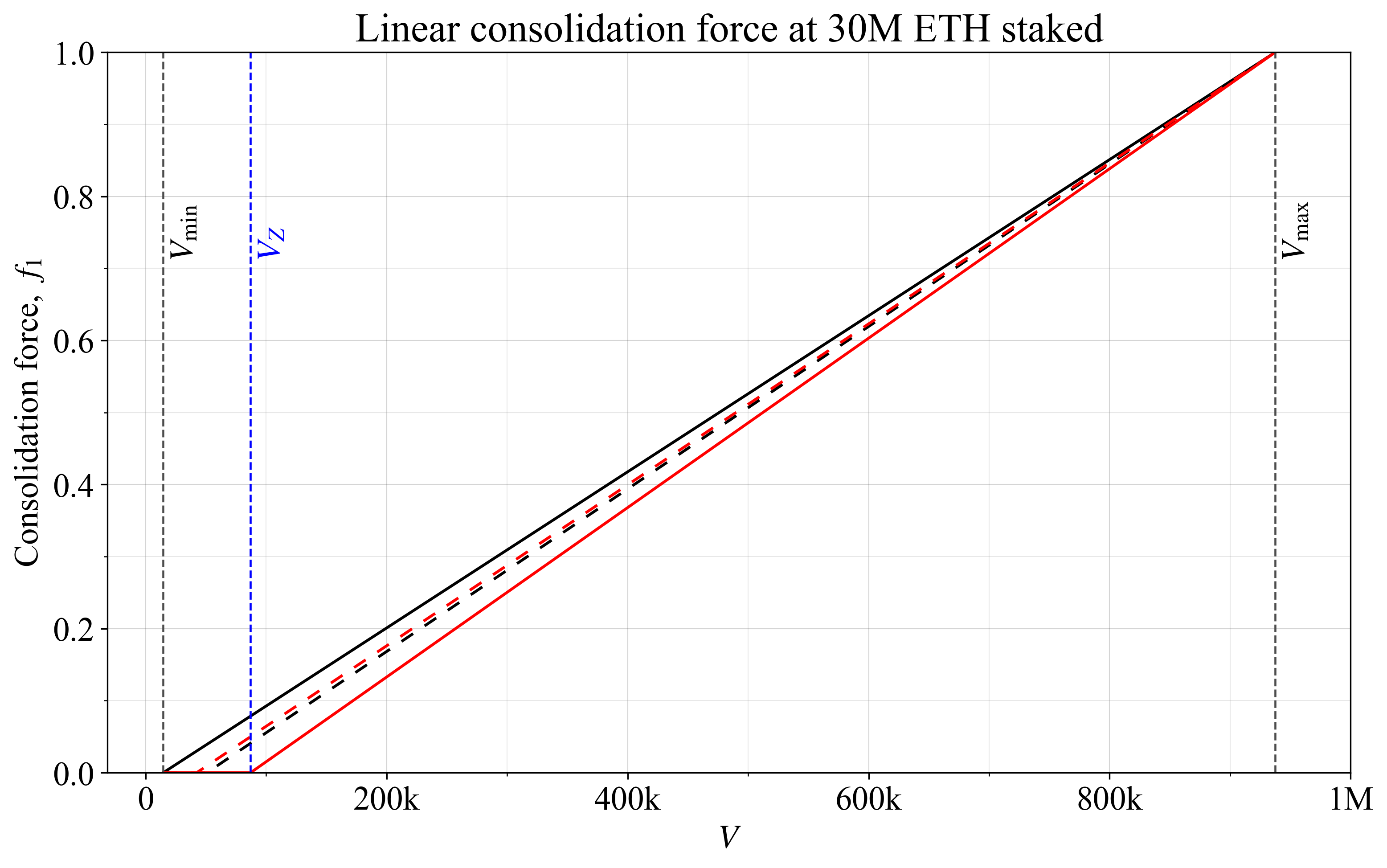
Figure 1. Four examples of a linear consolidation force f_1, reaching zero at different validator counts.
2.2.2 Sigmoidal shape
A more versatile alternative begins with the first step as previously:
A second step is then applied to produce a sigmoid:
The parameter t controls where the sigmoid’s main transition occurs, and the power (here 2) adjusts its steepness. Figure 2 illustrates a sigmoid (power 2) that pushes the transition to the left, close to V_Z, by settng t=5. The start point was set to V_{\text{start}} = (V_{\text{min}}+V_Z)/2 (as in the dashed black curve of the previous Figure 1).
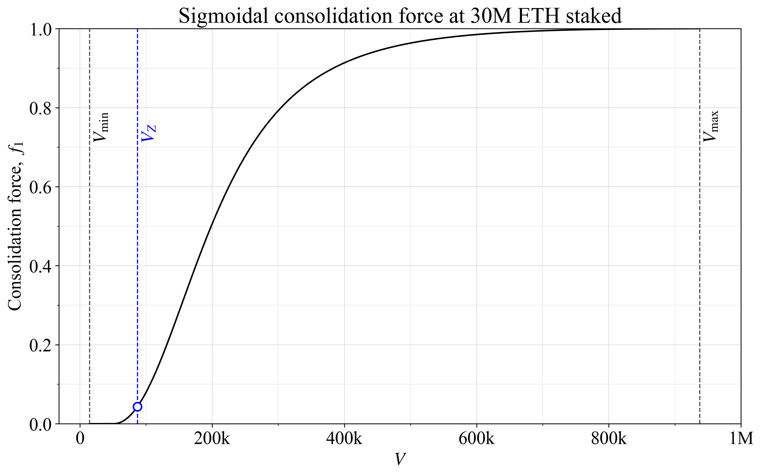
Figure 2. A consolidation force with a sigmoidal shape, which has an adjustable steepness and transition point.
A steep sigmoidal consolidation force is more relevant to consider for individual incentives, where the f_1 magnitude regulates the yield differential between stakers and thus represents the consolidation incentive. For collective incentives, the slope of the f_1 magnitude instead represents the consolidation incentive. A compromise that can be used both for collective and individual incentives would be to mix the linear and sigmoidal shape.
2.2.3 Mixed shape
A mixed shape can be generated through the equation
The first part of the equation creates the sigmoidal shape, which is weighed by w against the linear shape in the second part. Figure 3 shows an example with an equal weighing w=0.5, once again with t=5 and the same V_{\text{start}} at the halfway point between V_{\text{min}} and V_{\text{start}} as previously. Note the rather fixed slope between 400k and 1M validators, associated with the linear shape.
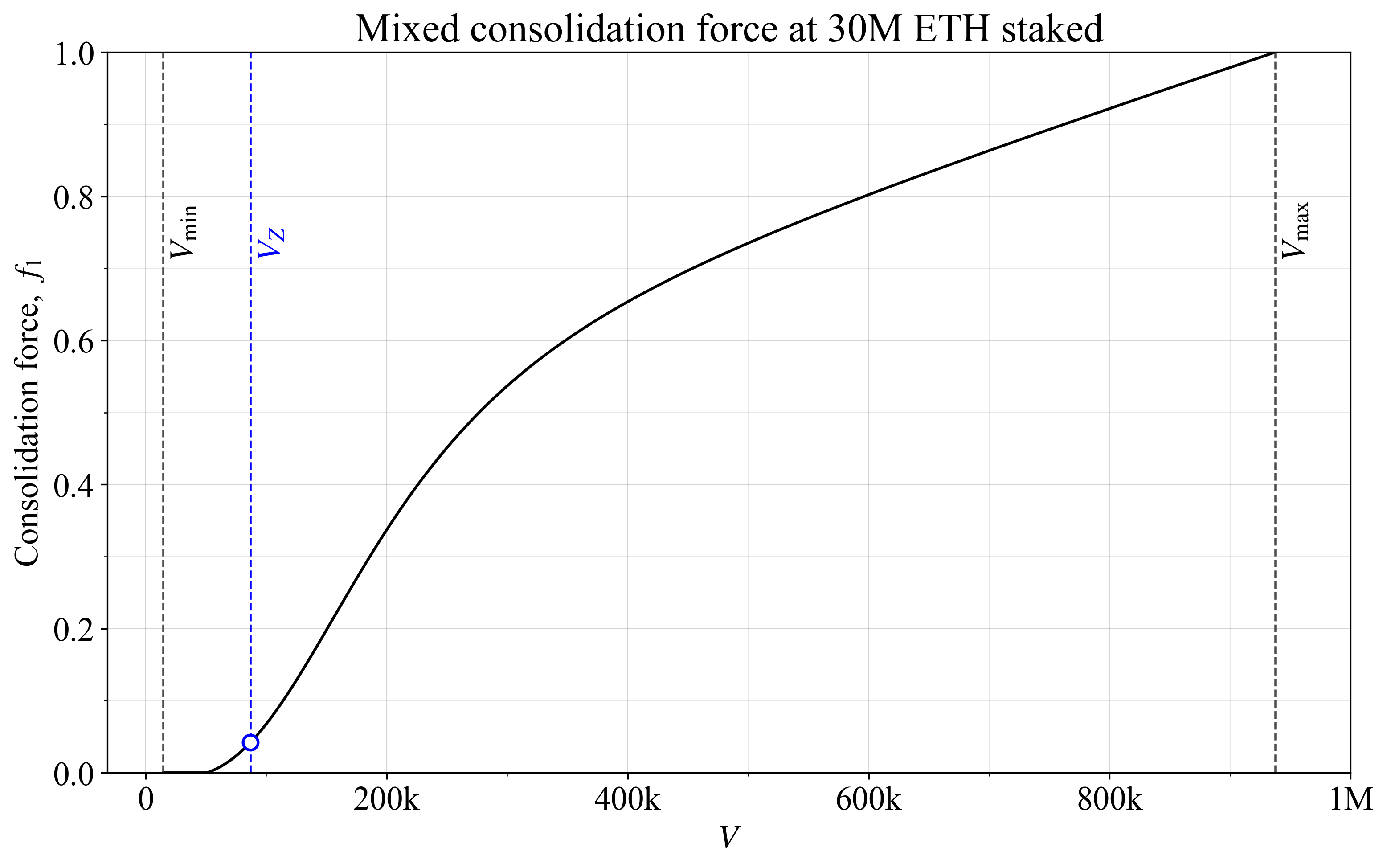
Figure 3. A mixed consolidation force, weighing together the linear and sigmoidal f_1 curve.
Just as with the other options, a question to consider is whether f_1 should go to zero already around V_Z, or if it is reasonable to leave some small incentive in place throughout the full range. The latter option seems perhaps more attractive since, presumably, some individual incentive must remain in place under equilibrium. In other words, setting the individual incentive to zero at V_Z precludes this point from being reached if it is not otherwise a profitable option for staking service providers (SSPs). But the existence of any remaining collective consolidation incentives at V_Z can then also factor in.
2.3 Fixed or dynamic schedule
Consolidation incentives can have a fixed or dynamic schedule. Under a fixed schedule, a specific validator composition at some quantity of stake will give a specific f_1 as illustrated in Figures 1-3. With a dynamic schedule, there is also a time component, and f_1 will adjust slowly towards its stipulated target. The dynamic schedule can still have the same type of f_1 curve as a target, as previously exemplified for the issuance reward curve, with a typical gradual shift captured here.
The most natural choice is to have a fixed schedule with no time component. The reason is the same as when it comes to the reward curve: the focus is the effect in the long run. The curve can capture the sought balance between fairness and the incentive to consolidate without involving time as a parameter. However, if the protocol wishes to puruse more extreme measures, such as for example forcing a Zipfian distribution by otherwise letting the f_1 of the individual incentive (f_1f_2f_y) approach infinity, then a dynamic schedule is required. But such a strategy can lead to very high yield differentials between small solo stakers and delegating stakers under equilibrium. It is then instead preferable to strike a balance between the need for consolidation and the need for fairness via f_1 curves similar to those outlined in this post.
Should there be particular concerns around stakers temporarily altering the validator composition, for example in response to changes in MEV or as a means for discouraging other stakers, it is of course possible to let the change to the long-run force be applied gradually when a shift occurs. Besides additional complexity, an additional risk is that if the f_1 does not adjust quickly enough with changing circumstances, there is a risk of stakers “overshooting” the natural equilibrium consolidation level.
3. Force distribution f_2 for individual incentives
The force distribution f_2 distributes the consolidation force across the validator set, forming individual incentives. In the baseline “attenuating” mode, a validator with a specific f_2 receives an individual yield attenuation of f_1f_2f_y. In the boosting mode it receives a boost of f_1(1-f_2)f_y under the same f_2 curve, but this section will be centered on the attenuating mode (a further review of mode is presented in Section 5 with a comparison in Table 1). Validators of the maximum size will generally have f_2=0 and thus no attenuation. Validators of the minimum size will generally have f_2=1 and thus receive the maximum attenuation f_1f_y. In essence, given a yield differential f_1f_y between the biggest/most active and smallest/least active validators, the role of f_2 is to determine the effect on all validators in between.
There are two main avenues for how to compute f_2 for each individual validator:
- AID (Section 3.1): incentives-differential based on an applied notion of fairness such as related to activity rate or validator size. This solution is the easiest to implement.
- CID (Section 3.2): cumulative incentives-differential as an overlay on top of AID, that distributes the designed incentives based on a sorted list of validator sizes. This is an attempt to adjust rewards if certain validator sizes become too favorable, but it is more complex.
A third option “BID” (Section 3.3) attempts to strike a balance by computing both an AID and a CID, letting f_2 be a weighing of both.
3.1 AID
With AID, the protocol adjusts the yield based on risks assumed or space taken up by validators. A natural assumption is that risks vary with activity rate a (the proportion of the time that a validator is active as an attester), which in turn varies with validator size s. If the activity rates are not the same for validators when they attest to the available chain and the finality gadget, but still vary between validators for both attestation duties, a unified measure would need to be defined. This section will review four options for the f_2 curve:
- Sec. 3.1.1; f_2(a): attenuate the yield based on an estimate of assumed risks derived from a.
- Sec. 3.1.2; f_2(s): simulate a validator fee based on the size s of the validator.
- Sec. 3.1.3; f_2(a) or f_2(s) or f_2(a, s): rely on a log-scaled measure with equidistant reduction across either a or s or both.
- Sec. 3.1.4; f_2(a, s): use a weighed average of the first two options.
Section 3.1.5 finally compares the options and plots them.
3.1.1 Linear in a – neutral w.r.t. expected active stake
Define the activity rate of validator v as a_v. An intuitive solution favored previously is to let f_2 capture inactivity percentage by deducting the activity rate
The equation can be re-scaled to always have the force extend across the full range. Define the minimum possible activity rate as a_{\text{min}} and the maximum as a_{\text{max}}. The f_2 for a validator with activity rate a_v can then be computed as
The type of linear scaling of f_2 presented in the above two equations results in the following feature: since stakers pay specifically for inactivity, an agent with an endowment to be staked—realizing some specific expected active stake—is affected equally regardless of which exact distribution of validator sizes it selects. For example, an agent staking 4096 ETH using one 2048-ETH validator and sixty-four 32-ETH validators will get almost the same expected active stake as when opting to run four 1024-ETH validators, and thus almost the same f_2 on average across its stake. Any other combination yielding the same amount of active stake will yield the same average f_2.
With a focus on activity as risk, this seems like a natural solution. There are many nuances to the question of how activity rates and validator compositions actually translate to risk. Further dialogue with staking service providers could provide important perspectives and more elaborate measures.
3.1.2 Inversely proportional to s – neutral w.r.t. number of validators
From the protocol’s perspective, should the two example distributions in Sec. 3.1.1 actually be treated equally? The second option with 4 1024-ETH validators might seem better, given that the first option instead results in 65 validators. It is preferable to be able to fully finalize the 4096-ETH endowment by providing space for only 4 validators in total in one slot, as opposed to requiring space for 65 validators. What would an equation that instead is neutral w.r.t. validator count look like? Define the size of a validator as s_v. The sought equation is then
with validators of size 32 receiving the full attenuation (f_2=1). This equation can also be re-scaled to always have the force extend across the full range:
The inversely proportional f_2 can be thought of as simulating a classical “validator fee”, and the mechanism is neutral with regard to the number of validators that some specific endowment is distributed across. The fee must be taken via an inverse relationship because of how the consolidation force is constructed to be deducted from the earnings. If the same f_2 was applied to every validator, a bigger validator would have to pay a higher nominal fee, given that its total rewards are higher. The inverse scaling rectifies that by weighing across stake. One way to understand the equation is to consider the outcome for 2048 ETH staked using any validator size. The total fee for 64 32-ETH validators then becomes 64 times higher than for 1 2048-ETH validator, the fee for 32 64-ETH validators becomes 32 times higher, etc (ignoring the re-scaling normalization). Another way to understand it is that f_1f_y comes to stipulate the validator fee for one 32-ETH validator. Running a 64-ETH validator costs the same in total as a 32-ETH validator, and thus f_1f_y must be halved when distributed across twice the stake.
In Orbit SSF with a 2048-ETH threshold, a_v and s_v will be linearly related, so the equation could then easily also be framed in terms of a_v:
However, this will not work if thresholding at for example 1024, or in Vorbit SSF with a more elaborate connection between validator size and activity rate, as illustrated in Figure 22 of that post.
3.1.3 Log-scaled – equidistant f_2 in log domain
While the inversely proportional scaling across s_v could lead to smaller validator sets, it might seem less “fair” than the linear construction across a_v. An agent in control of less stake might overlook its lower yield if the distribution specifically is designed to compensate validators for being more active, thus assuming greater risk. On the other hand, fairness could however also be constructed to reflect the strain that a staker puts on the protocol.
Note further that a distribution that is neutral w.r.t. expected active stake (Sec. 3.1.1) will give very similar outcomes for validator sizes ranging between 32-128 ETH (see also Figure 4 in Section 3.1.5). A distribution that is neutral w.r.t. number of validators (Sec. 3.1.2) will give very similar outcomes for validator sizes ranging between 512-2048 ETH. It might instead seem desirable for stakers with a compromise distribution where f_2 is affected equally at any point from the same log-scaled change to either a_v or s_v. Such a force distribution, scaled to span the full range, is
or
or a weighed combination of the two. This construction avoids the more extreme outcomes of the previous two ideas.
3.1.4 Weighing of linear and inversely proportional f_2
A fourth option is to weigh together the linear (3.1.1) and inversely proportional (3.1.2) constructions. A benefit is that both have a clear interpretation, which then extends to the weighed measure. The equation becomes
assuming a_{\text{max}} \neq a_{\text{min}}, with f_2=0 otherwise. The average shown in yellow in Figure 4 in the next subsection sets w=0.5. Note that this option is particularly useful when the relationship between a and s is less linear (e.g., Vorbit SSF).
3.1.5 Comparison of AID constructions
Figure 4 shows the four options previously presented using the validator sizes and activity rates of Orbit SSF thresholded at 2048, which is also s_{\text{max}}, such that a and s always are linearly related. Green and red $f_2$s are neutral w.r.t. estimated risk or occupied validator spots, and this gives fairly “lopsided” distributions. The log-scaled (blue) and average (yellow) distributions are less lopsided (at least from a log-scale perspective) and will see a more or less equal impact on f_2 when a validator doubles in size.
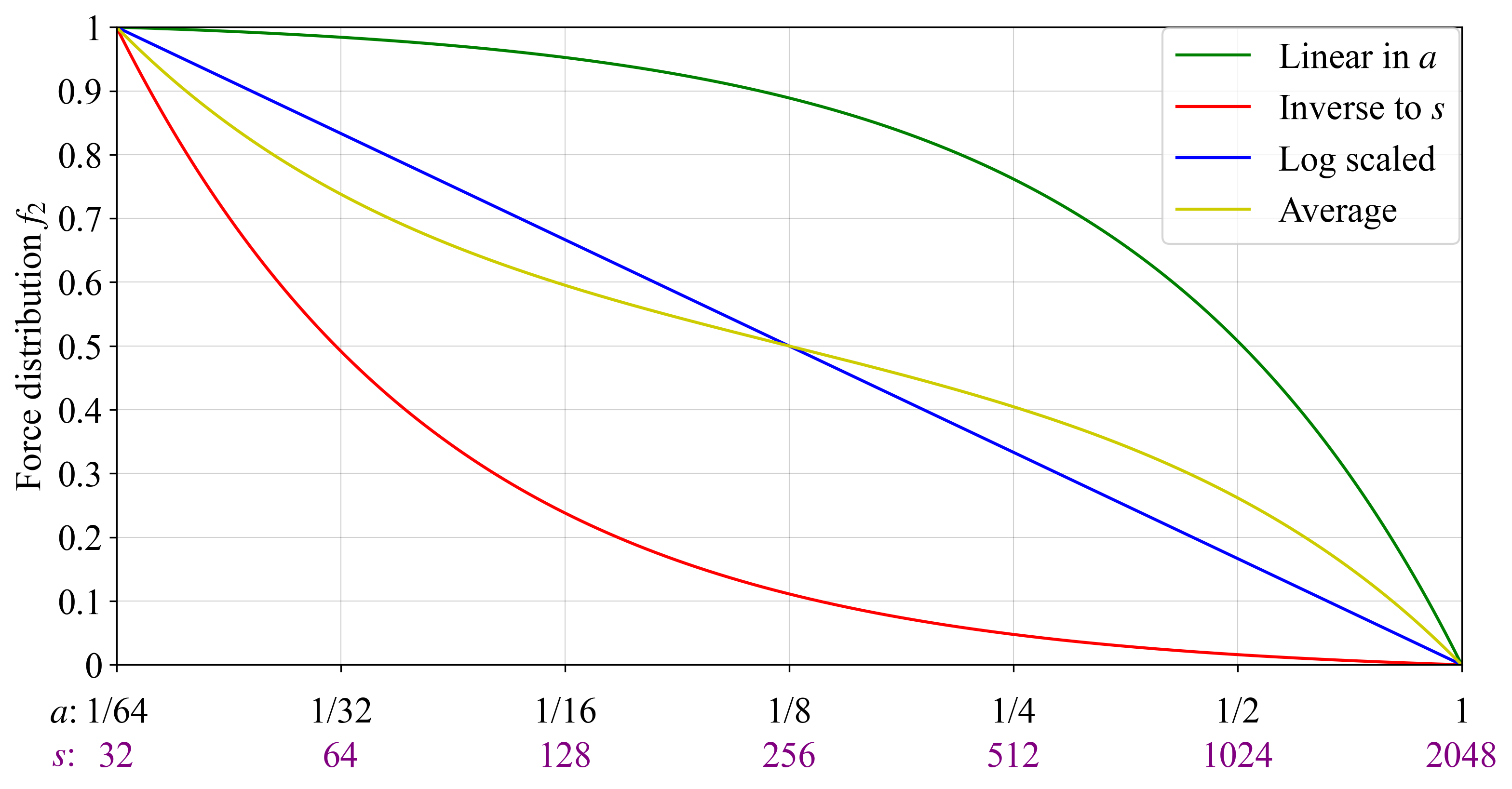
Figure 4. Four options for the force distribution f_2, plotted under a baseline Orbit SSF thresholding. In green, a distribution that is linear in a and neutral w.r.t. the expected active stake of some given endowment. In red, a distribution that is inversely proportional to s and neutral w.r.t. the number of validators used for some endowment. In yellow, the average of the green and red force distributions, and in blue a log-scaled distribution.
3.2 CID
Computing the f_2 via AID is simple and intuitive, but two things can be noted:
- If the mechanism does not model risks correctly, validators might congregate at sizes that produce the best risk-adjusted rewards, and the distribution may excessively diverge from some natural Zipfian state.
- The protocol’s priorities may change with consolidation level, focusing on how much space a staker takes up under low consolidation and focusing on fairness w.r.t. risk when the consolidation level already is good.
Points (1) and (2) can be addressed by applying a cumulative incentives-differential (CID) as an overlay on top of a specific AID policy. First, a neutral validator composition is defined and the applicable AID policy at this composition specified. Then, validators are sorted according to size and given the f_2 associated with their specific position in the sorted list.
A reasonable approach could be to define a Zipfian distribution of validators as neutral, such that the total ETH per log-spaced bin is fixed. Note here, that such a composition is a fair bit less consolidated than that generated from a Zipfian distribution of stakers, where each staker with more than 2048 ETH divides its stake into several big validators. Compare for example with Figure 2 in a previous post analyzing a Zipfian distribution of stakers.
Define a Zipfian distribution of validators as neutral and apply the CID across a log-scaled AID. Outcomes for various validator compositions with this specification are shown in Figures 5-10. As evident from Figures 5-6, when the validator distribution is Zipfian, a validator shifting its size will see its f_2 change just as under a pure log-scaled AID (blue line in Figure 4). If the consolidation level is less than Zipfian, the f_2 is closer to the inversely proportional distribution (red line in Figure 4). If the consolidation level is better than Zipfian, the f_2 is instead closer to the linear distribution (green line in Figure 4). The latter scenario is illustrated in Figures 7-8. Thus the protocol’s priorities shift with consolidation level, as discussed in point (2) above. To align even closer with that point in the case where the baseline Orbit weighting is not pursued, there would also need to be a gradual shift in focus from s to a as consolidation improves. One could consider (1-f_1)a+f_1s or something slightly more refined.

Figure 5. Force distribution f_2 under a Zipfian validator set plotted against the number of validators per bin.

Figure 6. Force distribution f_2 under a Zipfian validator set plotted against total ETH per bin.

Figure 7. Force distribution f_2 under a validator set that skews larger, plotted against the number of validators per bin.

Figure 8. Force distribution f_2 under a validator set that skews larger plotted against total ETH per bin.
If validators congregate at some specific size, it could imply that this size offers the best risk/reward. The force distribution will then automatically adapt, with the goal of stipulating a “fairer” yield for validators. An example is provided in Figures 9-10, with two peaks in validator sizes and a corresponding reaction in the force distribution. For illustrative purposes, the example is rather pronounced. In reality, there would likely be more subtle peaks and valleys, and thus more subtle changes to the f_2.
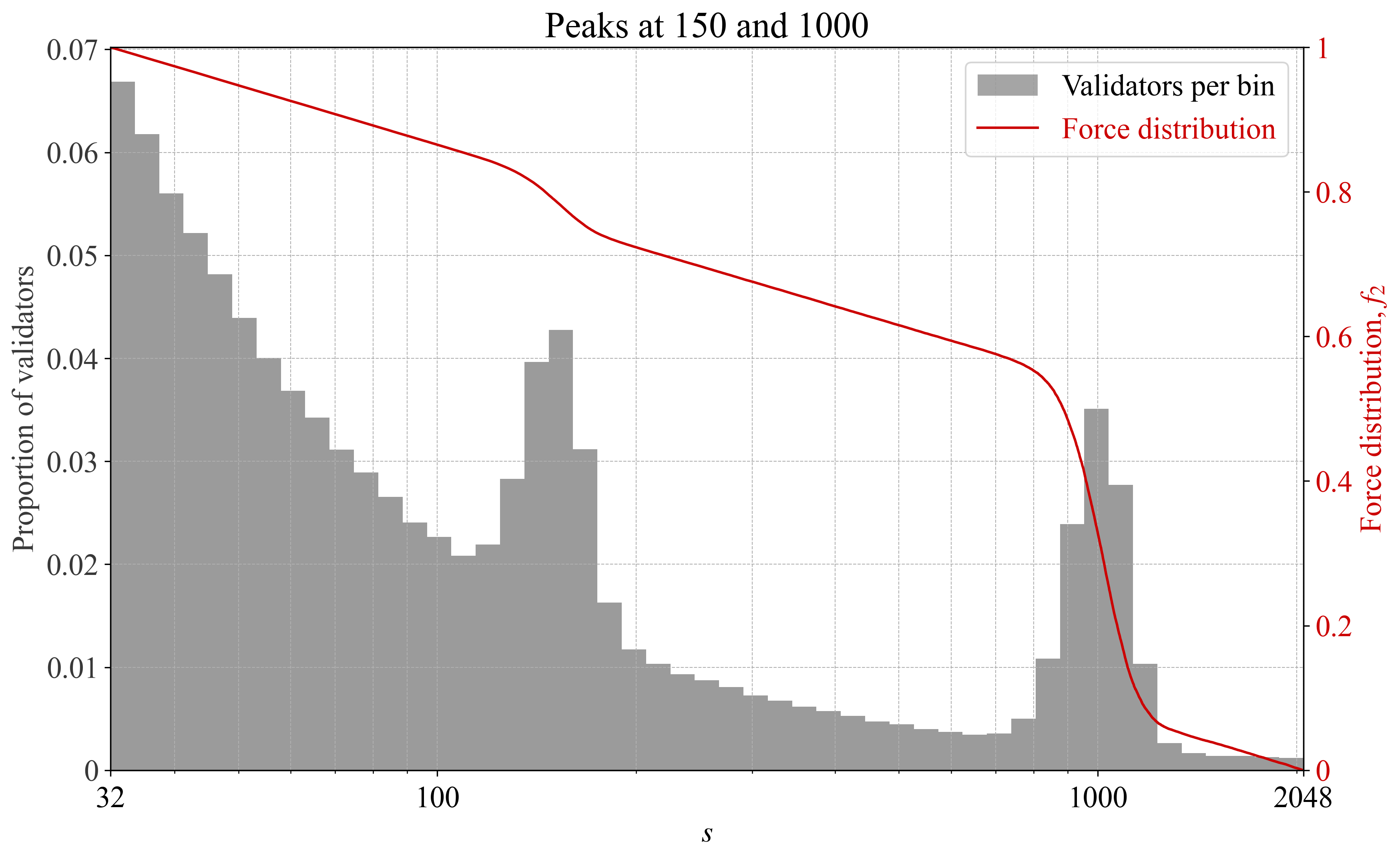
Figure 9. Force distribution f_2 under a validator set with local peaks, plotted against the number of validators per bin.
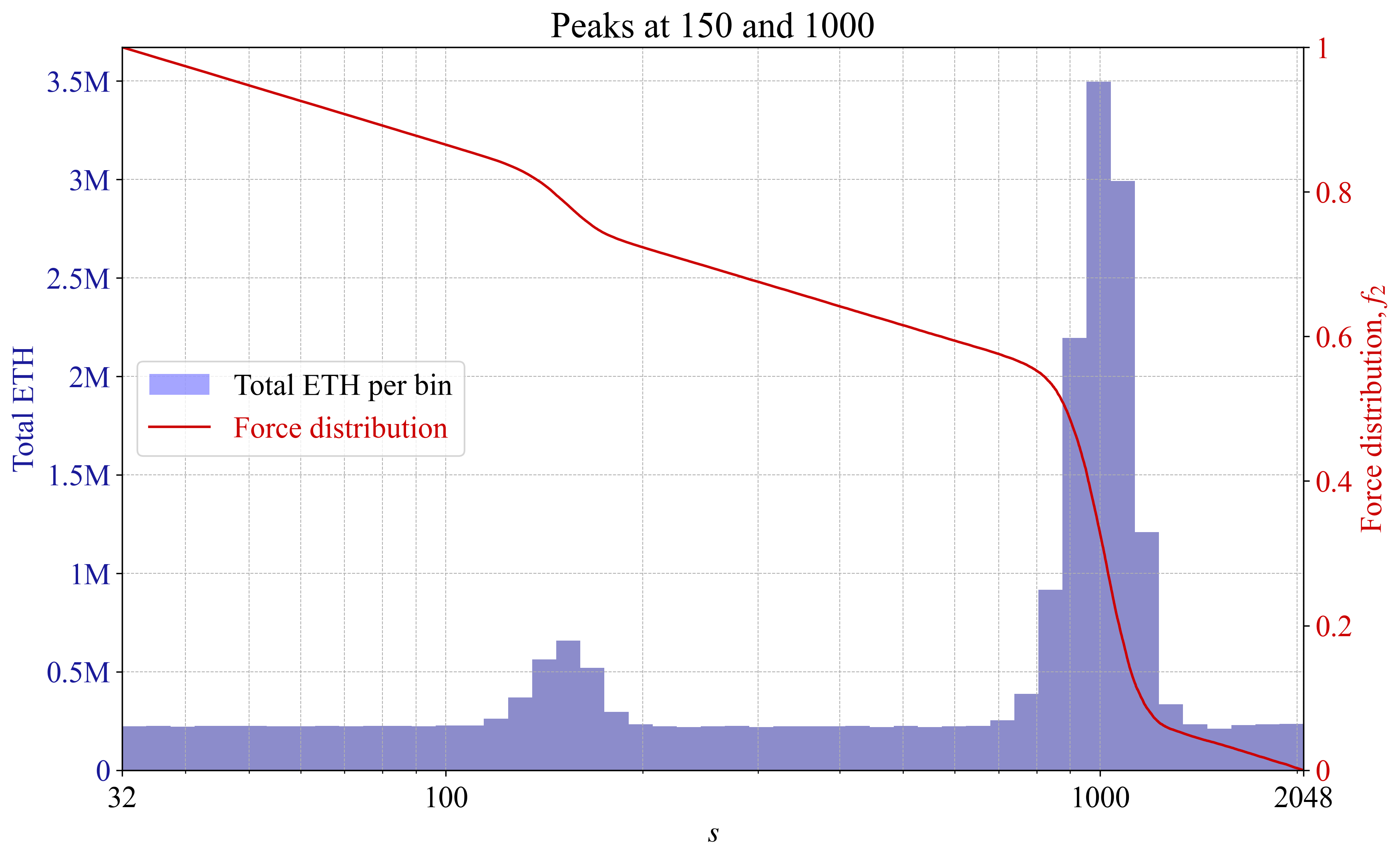
Figure 10. Force distribution f_2 under a validator set with local peaks plotted against total ETH per bin.
It might be beneficial to use a discretized measure of validators’ active balances at the boundaries of 32 ETH and 2048 ETH, to avoid micromanagement of balances. For example, all validators between 32-33 ETH and between 2040-2048 ETH might receive the same f_2, computed as the mean of the lowest and highest f_2 among validators within the range. Discretization at other ranges can be considered for computational reasons, but would presumably only lead to more micromanagement of balances.
Since CID introduces additional complexity, its benefits must be significant if it is to be adopted. It might then seem reasonable to first ship a pure AID if the overall strategy is to be pursued. The CID overlay can always be introduced if necessary at a later time.
3.3 BID – balancing between AID and CID
Naturally, a mixed measure of AID and CID, here referred to as BID, can be considered. This is an attempt to avoid problematic aspects of both variants when used in isolation. Both an AID f_2 and a CID f_2 are thus computed for the validator, and the final f_2 is a weighing of the two. It would then seem natural to use the AID underlying the CID as the measure for the AID.
4. Consolidation force scale f_y
The consolidation force scale f_y determines how much the yield should change given a consolidation force between 0 and 1. It can also be used for scaling total yearly issuance, then denoted f_I. This is the final parameter of the three used for consolidation incentives. Recall from previously that in the attenuating mode, the full equation for collective incentives is
and for individual incentives it is
The appropriate f_y will depend on the currently offered yield, how much MEV that is available relative to the yield, perceived risk of being active as a staker, the composition of the staking set, etc. Factors such as the existence of MEV burn at the time of adoption can therefore influence the appropriate scale (see further discussions in Sections 4.2 and 4.4 below).
Too weak consolidation will not sufficiently encourage consolidation. Too strong individual incentives will be interpreted (rightfully so) as Ethereum treating smaller validators unfairly. Strong collective (and individual) incentives can lead to frictions among consensus participants if the action of one party can have great influence on the yield of another party. For example, if there are no individual incentives, and some SSPs deconsolidate to lower their risk while significantly reducing yield for everyone, this might lead to particularly strong frictions.
Four designs of f_y are outlined in the following subsections. The right approach will depend on the shape of the reward curve, and a change in issuance policy could thus influence which approach that is the best.
4.1 Fraction of the issuance yield
One approach is to scale by a fraction of the issuance yield
or correspondingly by a fraction of the issuance
Setting k_1=0.1 gives a 0.1% reduction in yield if the issuance yield is 1% and the force is 1.
The idea behind using a fraction of the issuance yield is that the equilibrium staking yield implies something about the risks of staking. If the equilibrium yield is high, a larger incentive might be required to encourage consolidation than if the yield is low. Stakers are thus charged some fraction of their income for reducing their risk (or occupying consensus spots). One downside is that issuance yield is not the only reward currently befalling stakers: MEV accrues to all stakers equally and this income will not be reflected in k_1y_i. Another issue is that the equilibrium yield also compensates for other more general “costs” of staking (e.g., hardware) and those staking costs are much less affected by the activity rate of a validator.
4.2 Fixed ETH/year
Another idea is to derive the scale as a fixed ETH/year through
or correspondingly
Setting k_2=60\,000 would give a 0.1% reduction in yield at 60M ETH staked if the force is 1.
If rewards are dominated by MEV (including priority fees) and the MEV remains roughly constant, then this way of scaling the incentives will work rather well. The staking yield still varies with deposit size because the fixed MEV must be distributed to all stake. The consolidation incentive will thus adapt with the staking yield without attaching too much weight to the less relevant issuance yield.
4.3 Fixed yield, regardless of issuance and MEV
A third option is to specify a fixed yield component, i.e., simply
or correspondingly
Setting k_3= 0.001 would give a 0.1% reduction in yield if the force is 1.
With this design, the nominal incentive will remain the same, regardless of the level of the staking yield (if f_1 and f_2 stay the same). If risks associated with being active as a staker remain constant, such that an equilibrium shift in yield does not imply a change to such risks, then this approach can be reasonable. It could also be suitable if the stake supply curve is rather flat and remains fixed. In this case, any change in MEV would be offset by a shift in deposit size, such that the equilibrium yield also remains fixed. A probabilistic argument can also be made for the design under a shifting supply curve, with a reward curve rather similar to the present one. An equilibrium at a high deposit size is then likely associated with an increase in MEV (because the supply curve would otherwise need to fall improbably low). The suggestion is that the most probable staking yield across deposit size is more fixed than what the reward curve alone would indicate.
4.4 Mixed f_y – fraction of y_i and fixed ETH/year
The force scale can be a mix of several of the previous suggestions, because they can complement each other. For example, the specification could be
or correspondingly
With the previously discussed settings and D = 60\text{M} ETH, if an issuance yield of 1% is offered at this deposit size, the outcome would be
thus 0.2%. The suggested mixed f_y can be regarded as an attempt to relate the consolidation incentive to both issuance and MEV yield, and thus to the overall staking yield, which seems like a desirable objective. This can be expressed a little differently, as
where y'_v is k_2/D, but reframed as an estimate of the MEV yield. In this formulation, k_1 regulates the strength of both y_i and y'_v—that together represent the staking yield. The MEV cannot currently be directly computed (“seen”) by the protocol, and would thus need to be updated outside of its domain. What could be considered is to have some agreed-upon way to compute y'_v, or for that matter to leave it fixed at the current level and commit to only change it if MEV burn is instituted. As an example, say that the force scale is set to k_1 = 20\% of the staking yield. The equation then becomes 0.2(y_i + y'_v). As a guideline, 310k ETH of MEV was distributed via MEV boost during 2023. It fell to around 220k ETH in 2024. Relying only on MEV boost, a rough long-run estimate of y'_v at 34M ETH staked could thus be
The estimate always pertains to yearly MEV and not MEV yield specifically. The deposit size D is known by the protocol, just as issuance yield, and need not be estimated. The issuance yield under ideal consensus performance at 34M ETH staked is around 2.85%, and the maximum incentive would thus be
i.e., 0.7%. This is a rather strong incentive, albeit only activated under a completely deconsolidated validator set (f_1=1). Even if there is a desire to ultimately pursue such a strong incentive, it might still be reasonable to start out softer, at k_1\leq 0.1.
5. Attenuating, boosting, or issuance-neutral incentives
There are three possible modes for individual incentives: attenuating, boosting or issuance neutral (relative to the reward curve); and two modes for collective incentives: attenuating or boosting. Collective incentives can never be issuance neutral since the point of the mechanism is to collectively (for everyone) adjust rewards with consolidation level. This section reviews benefits and downsides of the possible modes and also highlights equivalences between them. The conclusion is that attenuating incentives are the most preferable, and that issuance-neutral incentives are the second best option (applicable to individual incentives). For clarity, Table 1 specifies the baseline equation for the different modes, assuming that f_1 and f_2 are computed as in Sections 2-3, with the issuance-neutral equation described in Section 5.2.1.
| Column 1 | Collective | Individual |
|---|---|---|
| Attenuating | -\,f_1f_y | -\,f_1f_2f_y |
| Boosting | +\,(1-f_1)f_y | +\,f_1(1-f_2)f_y |
| Issuance neutral | -\,f_1(f_2-\frac{\sum_{i} f_{2(i)}s_i}{\sum_{i} s_i})f_y |
Table 1. Baseline equations for the different modes for collective and individual incentives, when the f_1 and f_2 are computed as described in Sections 2-3, and with issuance-neutral equation described in Section 5.2.1.
5.1 Optimal mode for collective incentives
5.1.1 Equivalence
The mode of the collective incentive is of less importance than the mode of the individual incentive, since the attenuating and boosting modes in the collective incentive can be made equivalent. Let a higher reward curve A be attenuated and a lower reward curve B be boosted, and set the difference between them as the force scale f_y (ignoring complications regarding its computation). Further let y_c = f_1(V)f_y for A and y_c = (1-f_1(V))f_y for B under any V. Then, y_i-y_c for A will equal y_i+y_c for B:
The equality is trivial to achieve, and the chosen mode will then have no influence on the actual incentives for consensus participants.
5.1.2 Clarity
However, there is still some relevance to the mode. With an attenuating mode, the reward curve comes to stipulate the maximum possible issuance—an important feature to have plainly encoded. With a boosting mode, the maximum possible issuance can still be deduced, but it requires adding f_y to the reward curve. The reward curve then instead stipulates the minimum possible issuance under ideal performance when the staking set is deconsolidated—a somewhat less important feature. While the minimum possible yield is relevant both to stakers and as a general design criterion, the actual outcome is influenced also by luck in special duties assignments (e.g., block proposals), the actions of other consensus participants, etc. In either case, the minimum possible yield under ideal performance can still be calculated for attenuating incentives by deducting f_y.
5.1.3 Impact of re-parameterization
If the collective incentive is re-parameterized without altering the reward curve, it will affect the maximum issuance under boosting incentives and the minimum issuance under attenuating incentives with ideal attestation. In this case, for boosting incentives, the two possible outcomes are an increased maximum issuance (very sensitive) and a decreased maximum issuance (less sensitive). For attenuating incentives, the two possible outcomes are an increased minimum issuance under ideal performance (less sensitive) and a decreased minimum issuance under ideal performance (sensitive). Politically, having to increase the maximum issuance (or alter the reward curve) to achieve stronger collective incentives would likely be the most problematic. However, a reduction to the minimum would also be politically sensitive. This indicates that boosting incentives make future changes more socially costly.
As an aside, note that any premeditated change to collective incentives is problematic. Developers should encode the utility-maximizing incentive from the beginning. If it is known or suspected that f_1 or f_y will under some outcomes be adjusted, for example, a decreased boost under good consolidation, then the collective incentive to consolidate does not actually exist in the first place (c.f. the ratchet effect in production strategy).
Another thing to consider is re-parameterization due to changes in y'_v. If pursuing the parameterization in Section 4.4: f_y=k_1(y_i+y'_v), the maximum or minimum can change if y'_v changes. Once again, the sensitivity to increases and decreases must be considered, in particular the downside of having an increase in peak issuance any time y'_v increases.
5.2 Issuance-neutral individual incentives
5.2.1 Overview
Before comparing modes in individual incentives, the issuance-neutral mode will be presented. In the attenuating mode, f_2 is in the range 0-1, with small/inactive validators close to 1 and big/active validators close to 0. The consolidation incentive y_c derived from f_1f_2f_y is then subtracted from the targeted issuance yield for each validator. The “issuance neutral” approach computes a global linear displacement f'_2 = f_2-d such that aggregate issuance is left unaffected, while preserving the yield differential between small (inactive) and large (active) validators. This ultimately boosts the yield for large/active validators through a negative f_2 and attenuates it (but relatively less) for small validators, with a (smaller) positive f_2. Specifically, the mean of all f'_2\text{s} when weighted by size becomes 0. Let s_i be the size of validator i and f_2(i) its force distribution. The issuance-neutral displacement d can then be computed from the equation
Given that d applies equally to all validators, it can be understood as reflecting a collective incentive. In this context, it is however better described as an “anti-collective incentive”. Whatever aggregate shift in yield the attenuating or boosting individual incentive would produce, the variable d restores—acting equally for everyone—leaving the aggregate unaffected by consolidation level. Observe that this implies that boosting and attenuating individual incentives also contain some collective incentives—a boosting individual incentive will increase the aggregate yield and an attenuating individual incentive will decrease it. The issuance-neutral approach removes any trace of collective incentives from the individual incentives.
The role of c in the joint equation for consolidation incentives y_c = f_1f_y(c+f_2) can be compared with the role of the displacement d imposing f_2-d. The difference is that c is added whereas d is subtracted, and thus c \equiv -d. The collective part of the attenuating or boosting individual incentive is thus made explicit. It follows that if Ethereum uses both collective and individual incentives, they ought to be analyzed jointly. With this in mind, note that the boosting individual incentive in Table 1 from the beginning of the section ends up f_1f_y higher than then attenuating counterpart. They are thus separated by a collective component, and can be made equal through a shift f_1f_y.
Note that c is fixed beforehand and d is computed from—and varies with—f_2. The strength of c can be attuned to the protocol’s needs, but an adjusted strength can also be used for d. This adjustment can be stipulated as d' = dk_d. With 0<k_d<1, d' will see the collective part of the individual incentive positioned in between the issuance neutral and attenuating mode. Finally, it can be mentioned that to the individual validator, the aggregate is naturally of less direct importance, and the direct change to its f_2 is what matters—at least before any associated shifts in the equilibrium take place.
5.2.2 Rationale
Two benefits of issuance-neutral individual incentives can be identified, which are more relevant when combined with lower or no collective incentives. Firstly, protocol issuance will end up closer to the issuance level stipulated by the reward curve (regardless of consolidation level), which arguably improves design clarity. Secondly, one suggested approach to Ethereum’s issuance policy is to ensure that diligent 32-ETH solo stakers always receive positive regular rewards. At the same time, it is desirable to set the reward curve close to 0 at high deposit ratios. Issuance-neutral individual incentives allow Ethereum to compress the yield of small validators under low consolidation closer to the yield offered under good consolidation, such that the reward curve can be stipulated closer to 0 while still ensuring positive regular rewards. The f_1 is highest under low consolidation. At this point, there are more small validators than big, and the small validators rewards will only need to be reduced slightly to preserve neutrality (the few large validators’ rewards will at the same time be raised more substantially).
5.2.3 Simulations
To illustrate the compressed yield differential from issuance-neutral individual incentives for smaller 32-ETH validators, validator sets with smoothly varying Zipfianess were generated. A detailed description of the method is presented in Appendix C. Each validator set was generated by feeding the equally spaced uniform distribution u in the range [0, 1] into the equation
The composition of each validator set is in this equation governed by the exponent \alpha, where \alpha=-1 leads to a Zipfian distribution of validators. Appendix C.1 illustrates the effect of \alpha. The integral of the equation relates validator size V to deposit size D, and the closed-form solution can therefore be used to approximate the number of validators given a specific D and \alpha as:
Appendix C.2 presents the derivation. Figure 11 illustrates the effect of an issuance-neutral policy on 32-ETH validators at 80M ETH staked. It is created for \alpha between -6 and 2, at each point calculating the approximate V from the previous equation, generating the validator set at the specific \alpha, and computing the issuance-neutral displacement d. The linear f_1 that reaches 0 at (V_{\text{min}}+V_Z)/2 was used, and the log scaled f_2. The new issuance-neutral force f' for a validator with displaced force f'_2 then becomes f'=f_1f'_2.

Figure 11. Simulation of an issuance-neutral force aggregation for 32-ETH validators. The attenuating force can have f_2=1 for small validators at any consolidation level, and the maximum f is thus also 1 (thin black line). The issuance-neutral f'_2 (dashed blue line) only approaches 1 when almost no validators are of the minimum size, and after multiplication with f_1 (dotted blue line), the aggregated f' (black line) peaks at around 0.1.
As illustrated by the figure, f'_2 for 32-ETH validators will only approach 1 under consolidated validator sets. Larger validators then hold a clear majority of all ETH, and a small gain for them must be offset by a large reduction for small validators to preserve the yield differential under an issuance-neutral policy. But f_1 should at that point be set close to zero since the validator set already is consolidated, and a large yield differential would be perceived as unfair. The issuance-neutral aggregated force f' for 32-ETH validators therefore never exceeds 0.12. This allows the reward curve to be pushed much closer to zero while ensuring positive regular rewards than when using an attenuating policy (where f will approach 1 under low consolidation).
5.3 Optimal mode for individual incentives
5.3.1 Aggregate, individual, and equilibrium outcomes of different modes
Individual incentives should have a high yield differential when the validator set is deconsolidated and this is instituted by letting f_1 approach 1. A key problem under boosting individual incentives is therefore the rise in aggregate yield (further discussed in Section 5.2.1): deconsolidation is collectively rewarded. Note that this is opposite to how boosting collective incentives work (as evident from reviewing the equations in Table 1), where consolidation is rewarded instead (f_1 must then approach 1 if the validator set is consolidated). However, just as with the issuance-neutral incentive, the interaction of f_1 and f_2 must be accounted for. Define the average f_2 across the validator set, weighed by stake, as \bar{f_2} (this is in fact the same measure as previously computed for d). The average force per staked ETH \bar{f} by which issuance will be collectively boosted (after scaling by f_y) is shown in Figure 12, using the same validator distributions and shapes of f_1 and f_2 as previously for Figure 11. Since d offsets a 32-ETH validator with an f_2 of 0 (Figure 11) and the boosting incentive relies on 1-f_2 (Figure 12), Figures 11-12 appears identical, even though they illustrate two different concepts. The fall in 1-\bar{f_2} as consolidation level decreases moderates the actual collective outcome of the boosting incentive, with issuance even falling beyond 1M validators. This highlights that even with a boosting individual incentive, issuance may not rise substantially.
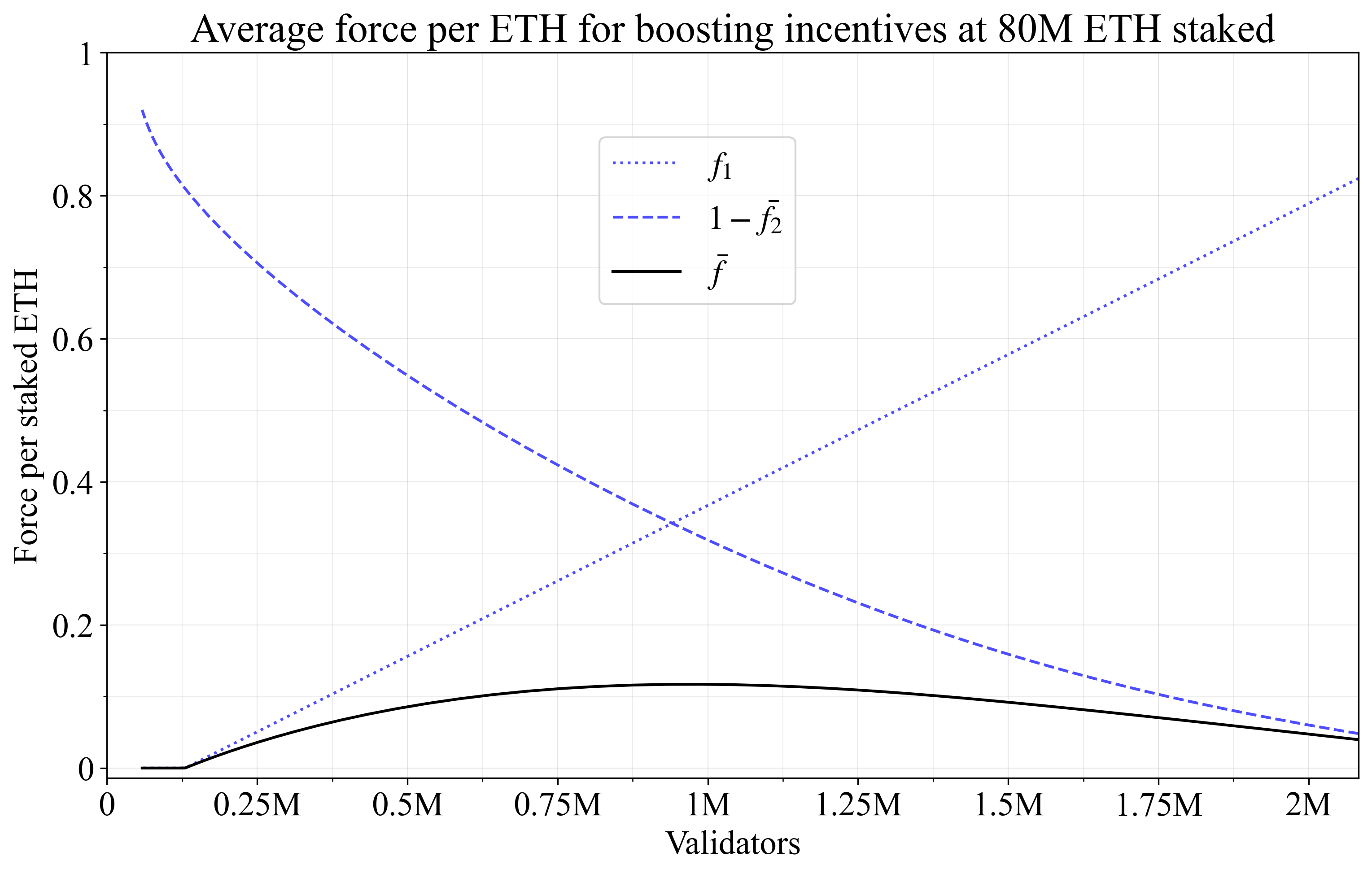
Figure 12. Analyzing collective effects of individual boosting incentives. The force per staked ETH peaks at around 0.12. This point, scaled by f_I, gives the maximum increase in issuance possible for the linear f_1 and log-scaled f_2 under the distribution of Appendix C.
Figure 13 instead shows the average force per staked ETH \bar{f} by which issuance will be collectively attenuated. Both f_1 and \bar{f_2} rise as consolidation falls, which is reflected in \bar{f}. The implication is that the “collective” portion of the individual attenuating incentive becomes much stronger than its boosting counterpart.
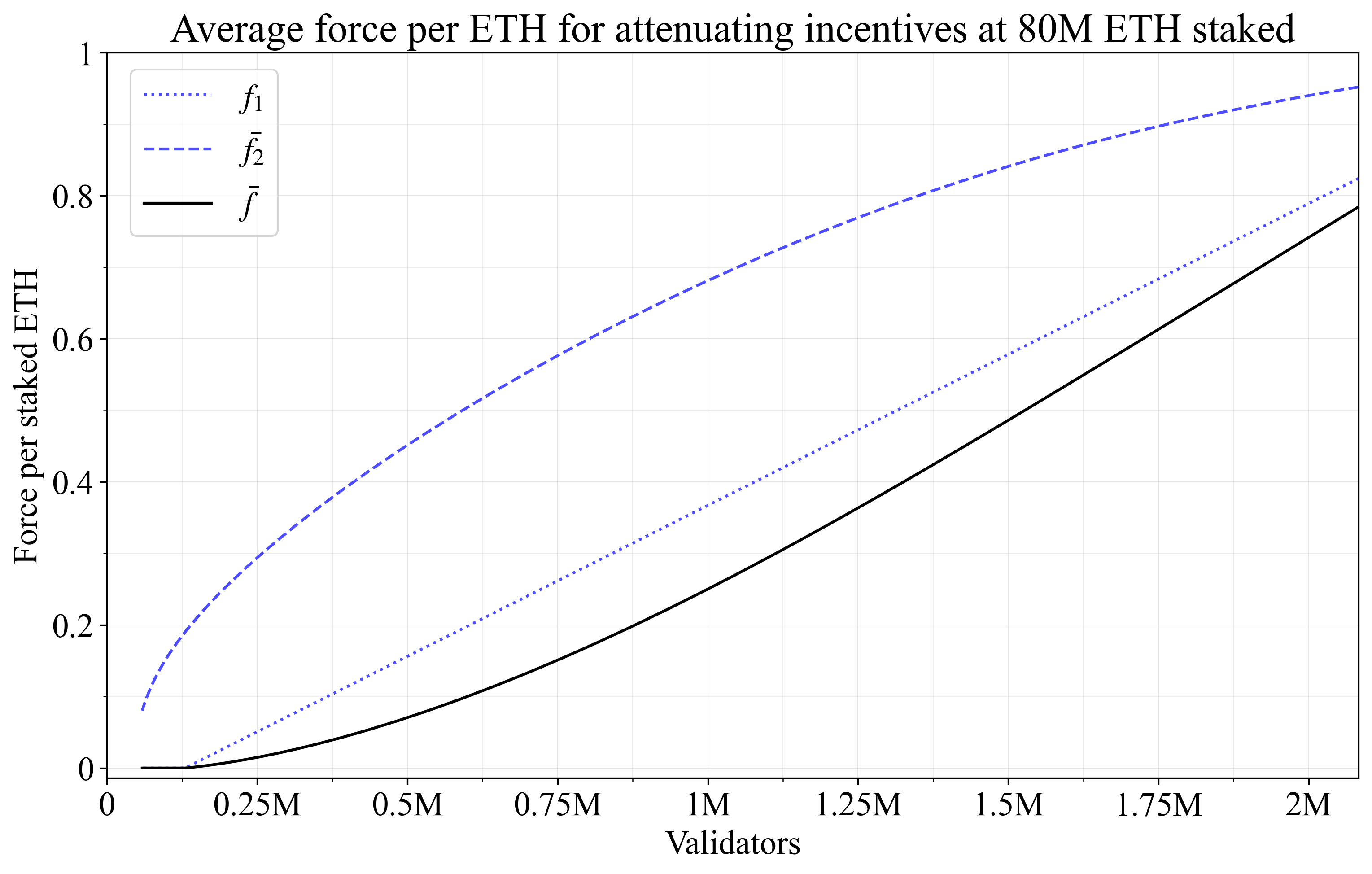
Figure 13. Analyzing collective effects of individual boosting incentives. The force per staked ETH approaches 1 as D approaches the maximum value, leading the issuance to be reduced by at most f_I.
Stakers can potentially actively deconsolidate to directly profit under boosting individual incentives. A staker holding many big validators who divides one of them into several smaller validators will see all remaining validators become more profitable. If the local derivative of the f_1 curve is large, and no attenuating collective incentives are in place, the gain among the remaining validators can come to offset the loss from the deconsolidated validator. For these reasons, if there are no collective incentives, certain implementations of boosting individual incentives would be very problematic. When there are collective incentives, their magnitude must be accounted for—recall from Section 5.2.1 that boosting individual incentives gives f_1f_y higher yield than attenuating individual incentives for all stakers (this is also evident by the fact that the black lines in Figures 12-13 sums to be equal to the dotted blue line). The general recommendation is to not pursue boosting individual incentives unless care is taken to never incentivize deconsolidation.
How about issuance-neutral individual incentives? It can be noted that since consolidation level will not affect issuance, the loss for a staker who deconsolidates a big validator will be precisely offset by an aggregate gain for all other validators. This alleviates concerns about a collective gain under deconsolidation, but a deconsolidating staker could still benefit. As f_1 increases, the yield will increase for big validators and fall for small validators, and a staker with many big validators may theoretically gain from deconsolidation—if the local derivative of f_1 is large. These concerns are however not comparable to those present for the boosting mode, and the issuance-neutral mode should not be ruled out given that it also brings benefits. Edge cases must however still be examined, but by adopting c>0 or changing d to d' with 0<k_d<1 (Sec. 5.2.1), such issues can be overcome.
Note that the equilibrium effect after stakers adjust their positions due to the change in yield will be smaller than the direct effect. An increase in f_1 from the initial deconsolidation will incentivize other stakers to consolidate, pushing f_1 back down. The equilibrium outcome can be a theoretical concern even in the attenuating mode. In this mode, a staker with many big validators can deconsolidate to push down the yield for small validators in the hope that some stop staking, leading to an increase in staking yield for the remaining big validators. While rather esoteric, the equilibrium outcome will at least be much more similar for the different modes than the direct outcome—the yield differential between big and small validators is kept fixed regardless of mode under the same f_1. However, the equilibrium outcome is more speculative, can be affected by the collective component in the individual incentive, and takes effect more slowly.
5.3.2 Collective concerns under various modes
The issues concerning collective incentives discussed in Section 5.1 apply also to individual incentives. This is due in part to the traces of collective incentives also present in individual incentives outlined in Section 5.2.1. Boosting individual incentives will also increase the maximum possible issuance. In particular, it is unfortunate that attenuating individual incentives will specifically push down the issuance of 32-ETH validators. The strong point of issuance-neutral incentives is that they do not increase the maximum possible issuance, while at the same time not worsening the outcome for 32-ETH validators too much in the worst-case scenario. This “compression” of the yield differential for 32-ETH validators was presented in Section 5.2 and illustrated in Figure 11.
5.3.3 Implications on discouragement attacks
Finally consider discouragement attacks with the additional twist of only targeting validators of a specific size. If small validators are targeted, some of them will stop staking and consolidation will improve. An attacker can thus gain from the collective consolidation incentive. An attenuating individual incentive will however lead to a direct increase in yield specifically for small validators upon consolidation, mitigating some concerns. Note further that an attenuating individual incentive makes it relatively more profitable for small validators to stage this attack (in terms of the direct effect), and a boosting incentive makes it relatively more profitable for large validators. If large validators are targeted, the collective consolidation incentive brings down the yield, so this attack is therefore only a concern under boosting individual incentives.
6. Concluding specification
A systematic framework for consolidation incentives in Orbit/Vorbit SSF has been presented. Benefits and drawbacks of various settings for the three consolidation forces f_1, f_2 and f_y were provided, and their optimal mode reviewed. Based on that analysis, the most beneficial settings will now be suggested, resulting in an overarching specification for how to incentivize consolidation.
§1. The post is centered around the attenuating mode with the main equation
The shape of the consolidation force is determined by f_1, the scale by f_y, the distribution between validators by f_2 (thus the f_2 is unique to each validator size) and the relative strength of collective incentives by c. The resulting consolidation incentive y_c differs with validator size and is used to update the target issuance yield for each validator:
§2. While it is not strictly necessary for f_1 and f_y to be the same for individual and any collective incentives, it is a realistic design goal to pursue.
§3. Let the shape of f_1 be based on the mixed equation, parameterized as outlined in Section 2.2 and captured in Figure 3. This is a versatile equation that can be adjusted to fit requirements as the architecture nears adoption.
§4. Use a fixed schedule for f_1 with no dynamic time component, for simplicity (Section 2.3).
§5. Let f_2 be a pure AID as a starting point. If relying on a Vorbit design, or generally any design with a less linear relationship between validator size and activity rate, use the mixed
presented as the yellow curve in Figure 4. Setting w=0.5 seems like a natural default choice (an even balance between focusing on active stake and occupied validator spots), but w>0.5 is also viable and arguably more fair. Even if the direction is to focus on active stake out of fairness concerns, w=0.8 should be sufficient to ensure that stakers opt for 2048-ETH validators over 1024-ETH validators when Orbit is thresholded at 1024, if they have the capital to do so. If the mixed measure is unnecessary, for example in Orbit SSF thresholded at 2048, it is also viable to use the log-scaled
presented as the blue curve in Figure 4. Two log-scaled f_2\text{s} computed both for s and a could also be averaged/weighed together under Vorbit SSF.
§6. The primary option is to let f_y be defined according to the mixed equation f_y=k_1(y_i + y'_v) with a long-run estimate in y'_v that is to be adjusted only after a substantial shift in MEV (e.g., after implementing MEV burn). It is preferable to start at a modest scale, i.e., k_1\leq0.1. Determining f_y based on a fixed ETH/year (Section 4.2) seems like the second-best option.
§7. The primary option is to use the attenuating mode both for individual and any collective incentive. However, the issuance-neutral approach also brings certain benefits due to its ability to compress the yield variability for small validators. It should be considered and analyzed further once a general design has been settled on. This analysis should rule out and parry edge cases of profitable deconsolidation outlined in Section 5.3.1.
§8. Consider using only the individual incentive, with no pure collective incentive, i.e., c=0. As noted in Section 5.2.1, the individual incentive still has a collective effect (directionally correct for attenuating incentives). If tensions in the staking set are not a concern, a relative modest collective incentive can be considered.
Appendix A – Approximated V under a Zipfian quantity of stakers
As outlined in Section 2.1, it seems intuitive to scale the strength of the consolidation incentives according to the Zipfianess of the staking set. For example, when the validator set is consolidated in line with a Zipfian staking set (when V \approx V_Z), consolidation incentives should be very small, to uphold fairness. It is therefore desirable to have an estimate of the number of validators under a Zipfian distribution. The number of validators V, assuming a pure Zipfian staking distribution with stakers consolidating all available stake, can be calculated in accordance with the equations of Appendix A in the post on Vorbit SSF. Given a specific D, the Zipfian staking set size is first computed as
where W denotes the Lambert W function and \gamma is the Euler–Mascheroni constant, approximately 0.577. If the minimum validator balance is 32 ETH, the Zipfian validator set size under full consolidation becomes
It would be desirable to have some simpler approximation of V_Z instead of these rather complex equations, given that Zipfianess in itself merely is a rough guideline and that the equation would be part of the consensus specification.
For large x, the Lambert W function behaves approximately as W(x) \approx \ln x - \ln \ln x. An approximation of N_z is therefore
where the numerator increases linearly with D and the denominator logarithmically with D. The linear term comes to dominate with large D, where the denominator changes relatively slowly. In the second of the first two equations, deriving V_Z from N_Z, the linear term once again dominates. A linear approximation should therefore come fairly close, but a log adjusted or loglog adjusted approximation would be more accurate. Figure A1 illustrates agreement with the Zipfian ground truth for the following four approximations:
Constants were selected to favor integers and simplicity. For example, setting the constant in the log adjusted equation to 19.9 instead of 20 brings the results slightly closer in line with the ground truth. However, a constant of 20 still keeps the difference roughly equal across the range at around 1000, and is perfectly sufficient for our purposes. The fourth option is included since all consensus clients already have implemented a function for taking the square root of D when computing the current reward curve. If the minimum validator balance changes, the general equations
and
can instead be used.
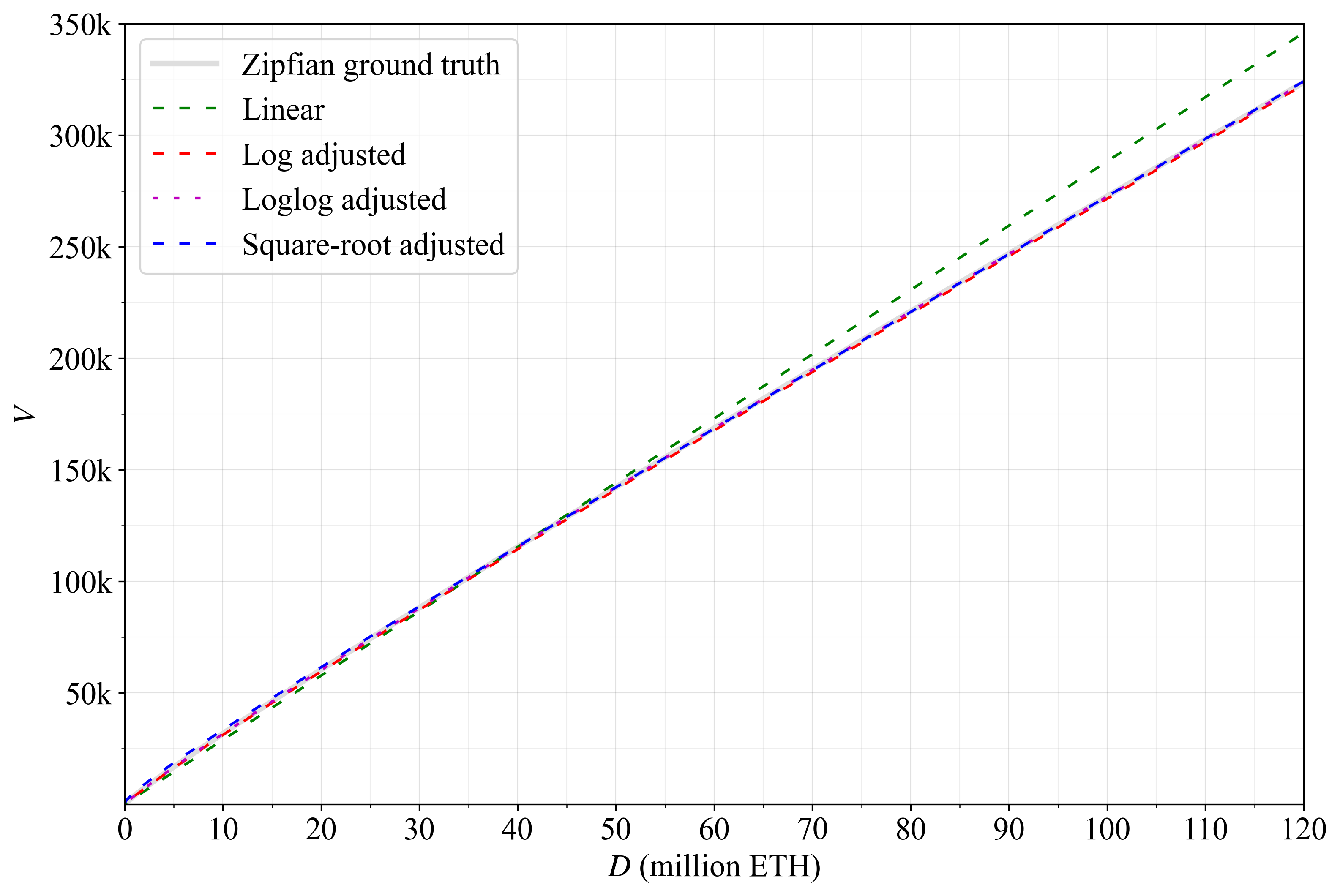
Figure A1. Various approximations of a pure Zipfian distribution.
Figure A2 shows the difference to the computed V_Z for the approximations in a more precise relative comparison. As evident, the loglog adjusted approximation comes very close, but the other approximations are also perfectly sufficient for the purpose of this specification.
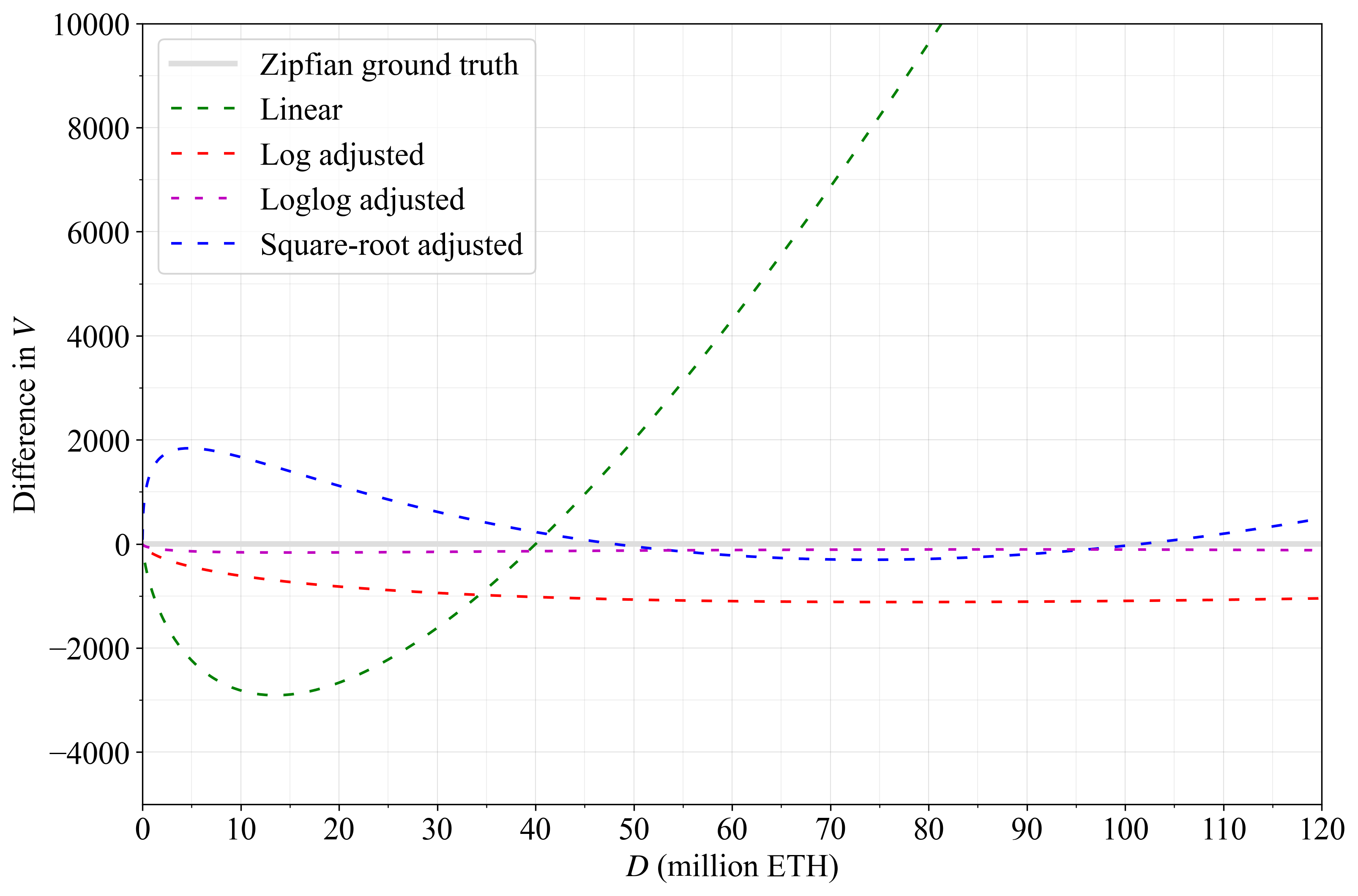
Figure A2. The difference between the outlined approximations and the ground-truth computation. The log adjusted equation produces a fairly even distance from the ground truth of 1000 validators and the loglog adjusted equation is nearly perfect.
Appendix B – Comparison with incentives in the Orbit SSF post
B.1 Collective incentives as a function of D_a
A comparison can be made with the incentives design previously proposed in the Orbit SSF post. That post outlines another strategy for collective consolidation incentives, where issuance depends directly on active stake I(D_a) as opposed to total stake I(D).
An equivalence must be based on the equation for the reward curve, such that the stipulated issuance at I(D) can be reflected back to the issuance at I(D_a) via the attenuation. Use the consolidation force scale defined in Section 4.1: f_I=k_1I with k_1=1. This means that the total attenuation I_c of issuance becomes I_c=f_If_1=If_1. The goal is to determine the f_1 that lets I - I_c become I(D_a) under the current reward curve cF\sqrt{D}, which is cF\sqrt{D_a} when using D_a. The equation is first expanded:
The consolidation force f_1 must then simply reflect back to the point D_a on the issuance curve. Therefore, if D_a/D stake is active, f_1 for the current reward curve must be
The equivalence is illustrated continuing from previously:
As a numerical example, say that half the stake is active. This means that the f_1-function must map f_1(1/2)=1-\sqrt{1/2}. Starting from cF\sqrt{D}=cF\sqrt{2D_a} (since half the stake is active), the operation becomes
The reader is encouraged to review the Orbit SSF analysis that also reviews similarities between I(D) and I(D_a), reaching results that can be linked to those presented here with the aid of the equations Appendix B.2. One detail worthy of further consideration is that f_1 is computed based on the number of validators V and not active stake D_a. When using V, the issuance curve will not be influenced by the Orbit specification. For example, should the threshold T in vanilla Orbit be adjusted, D_a would be adjusted, and thus issuance/consolidation incentives. There are both potential benefits and drawbacks of this.
When T=2048, the relationship between V and D_a is simple, given that the average validator size can be written both as
and
This means that the number of validators is
B.2 Collective incentives as a function of D
The appendix of the Orbit SSF post further suggests the alternative I(D)\frac{D_a}{D}, which is equivalent to using f_I=k_1I (from Section 4.1) with k_1=1 and f_1 = 1-D_a/D:
The possible link between D_a and V was further presented in Appendix B.1. A more general equivalence with references to the formulation in the Orbit SSF post is to set f_1 = 1-\delta(D_a/D).
B.3 Individual incentives
Concerning individual incentives, the Orbit SSF design can again be understood as f_y=k_1y_i with k_1=1. There is also a suggestion of limiting the scale to 25% of the issuance yield, i.e., similar to setting k_1=0.25. The equation corresponding to f_2 is linear in a, as in the first equation in Section 3.1.1, with the normalized version shown as the green line in Figure 4. The Orbit SSF post however suggests boosting yield as opposed to attenuating it, which explains the difference to the first equation in Section 3.1.1. Boosted individual incentives are highlighted as problematic in Section 5.3.1, due to the collective gain from deconsolidation. In isolation, they should thus be avoided, but it can be noted that the Orbit SSF post employs a strong collective incentives that compensates. The effect is similar to the compensatory effect discussed in Section 5.2.1.
There is finally also the notion of letting a term corresponding to f_1 reach 0 at some sufficient level of consolidation, here at D_a/D=0.8. This can be directly compared with letting the f_1-curve reach 0 once a Zipfian distribution of stakers has been achieved in terms of V.
Appendix C
C.1 Simulated validator distributions across \alpha
The equations for simulating a smooth variation in Zipfianess from Section 5.2.3 can be useful beyond this specific study. This appendix therefore provides some further insights and details for the previously presented equations. Begin with the generation of validators
and consider the Zipfian scenario when \alpha=-1. In this case, the exponent becomes 1/-1=-1, and the equation
The first uniformly spaced sample of 0 will produce a validator of size 1/(1/32)=32 and the last sample of 1 will produce a validator of size 1/(1/2048)=2048, as required. The inverse of the equal spacing in u serves to generate a harmonic series. The equation thus recreates the baseline approach in Section 2.1 of the Vorbit SSF post (this time applied to validators instead of stakers), but in a form that can be generalized to non-Zipfian distributions varying smoothly with \alpha. When \alpha=-1, around half the validators will have a balance below 64, as expected of the harmonic series. When \alpha<-1, validators are spaced tighter at low balances, leading to a less consolidated validator set, and when \alpha>-1, validators are spaced tighter at high balances, leading to a more consolidated set. Figure C1 shows the outcomes for \alpha=-1.9 (green), \alpha=-1 (orange), and \alpha=-0.1 (blue) in terms of total ETH located within each histogram bar. Note that \alpha=0 must always be avoided in simulation since 1/\alpha would go to infinity.
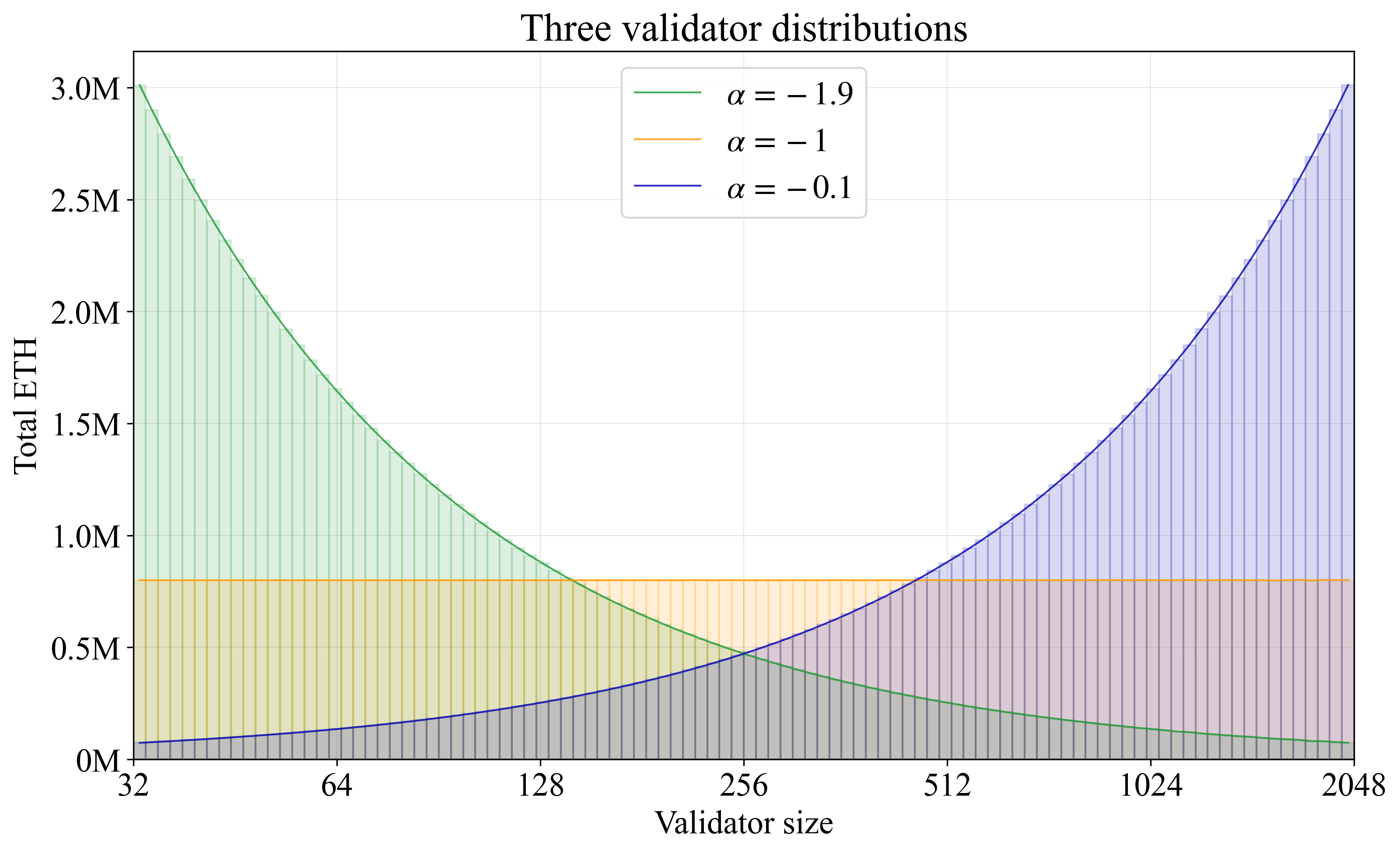
Figure C1. Histograms weighted by stake for three validator distributions at 80M ETH staked. A higher \alpha gives a distribution that is more consolidated, and \alpha=-1 gives a Zipfian distribution of validators.
C.2 Approximating V at any given D
The integral of the equation from Appendix C.1 can be used to capture the relationship between the number of validators (think of it as samples across the x-axis in Figure C1) and the total amount of ETH (the resulting area under the curve):
The closed-form solution is
The integral can be understood as stipulating the average validator size, given that it covers the range 0-1 in the uniform distribution u. It follows that the deposit size can be generated as D=VI_u and thus I_u=D/V. Substituting in gives
and the approximation can finally be solved for V as