FAQ: Ethereum issuance reduction

aelowsson · May 29, 2024, 3:20pm

FAQ: Ethereum issuance reduction

Overview

When it comes to the premise of reducing issuance, there are many important questions to consider. Having studied these questions extensively, I thought it would be fruitful to address them one by one, providing detailed answers as needed. I post on Ethresearch to facilitate debate, and will try to respond to any questions you may have (including new questions suitable for an extended FAQ).

Some concepts of staking economics that have just been discussed in passing previously are given a more extensive review. These include: time–quantity policies where the reward curve slowly drifts (and other potential endgame policies), distributions of reservation yields among solo stakers and delegating stakers, and the downsides of using a vanilla EIP-1559 mechanism to target some specific stake participation. Quick link to all questions:

It is beneficial to read the answers in the order that they are presented, but they still stand on their own.

FAQ

Why should Ethereum reduce its issuance?

Overview

At the most basic level, stake participation is growing beyond requirements for economic security, and paying people to do something that is not necessary always comes with downsides. To be more specific, there are two fundamental reasons for reducing issuance:

To reduce costs for users, including costs for hardware, risks and opportunity costs, taxes, etc. By maintaining the current reward curve, Ethereum compels users to incur higher costs than necessary for securing the network. Reducing issuance will improve welfare by eliminating implied costs that may very well amount to more than a billion dollars per year.
To improve Ethereum at the macro level. If everyone stakes, one entity or a cartel might come to exercise control over a large proportion of all ETH. This can reduce security since it becomes harder for the social layer to hold such entities accountable. The potential proliferation of liquid staking tokens (LSTs) may also impede ETH as trustless money, fostering monopolization and making Ethereum a less desirable blockchain to build on.

The answer will now take a closer look at these two aspects.

1. Reduced costs raise welfare

Review Figure 1 (example with more details here), featuring a hypothetical future supply curve in blue. The supply curve indicates the amount of stake deposited D at various staking yields y. It captures the implied marginal cost of staking. What that means is that every ETH holder is positioned along the supply curve according to how high cost they assign to staking, with their required yield reflecting that cost. Relevant costs include hardware and other resources, upkeep, the acquisition of technical knowledge, illiquidity, trust in third parties and other factors increasing the risk premium, various opportunity costs, taxes, etc. The area above the supply curve indicates the stakers’ surplus (what they actually gain). The area below the supply curve—the supply curve’s integral—indicates the costs assigned to staking (the marginal staker would not stake at a yield below the supply curve).

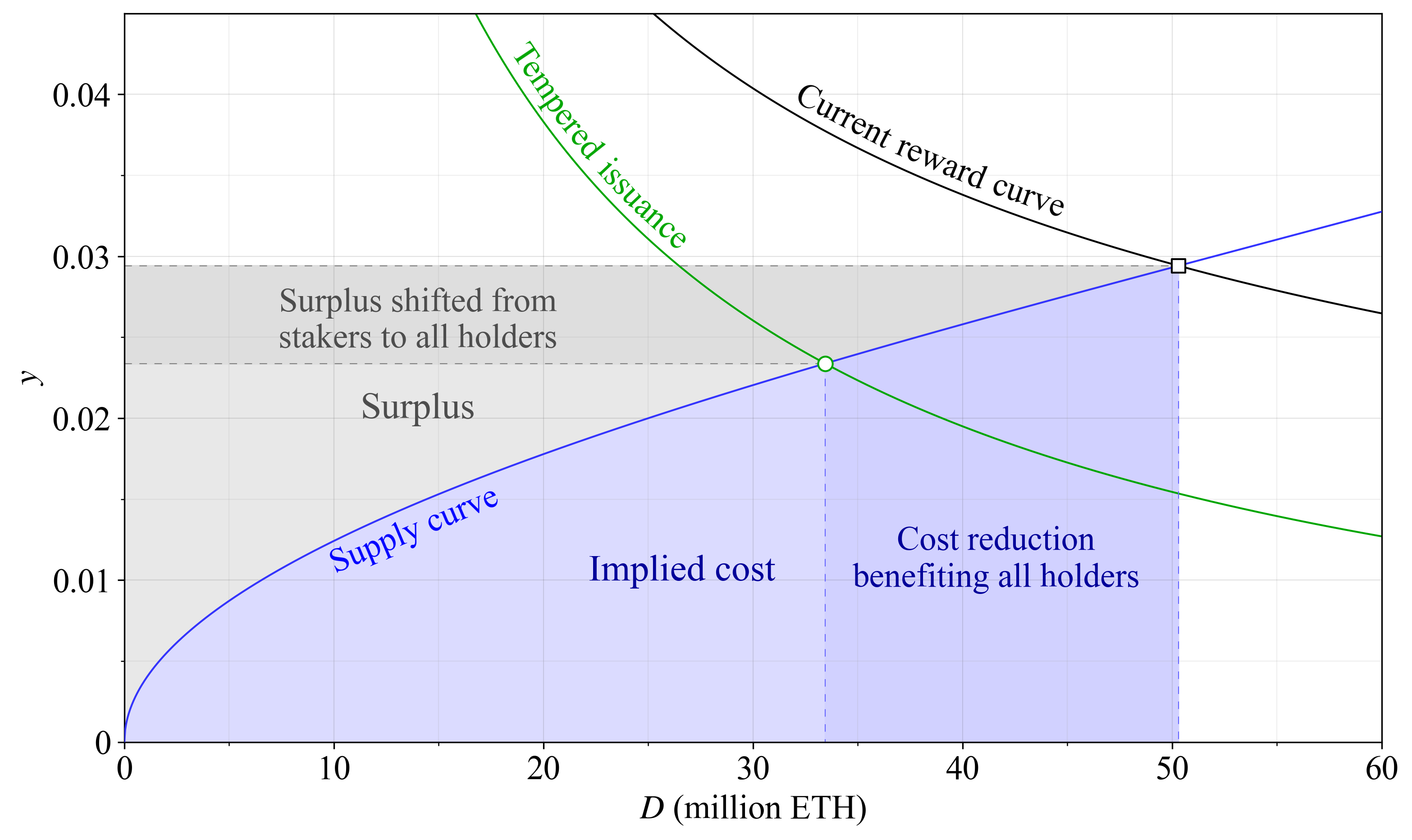
Figure 1. Implied cost (blue) and surplus (grey) of staking under a hypothetical future supply curve. A change in issuance policy shifts the equilibrium from the black square to the green circle. The cost reduction (dark blue) leads to aggregate welfare improvement as long as the protocol remains secure and decentralized, and the reduction in surplus (dark grey) simply shifts some utility from stakers to everyone.

Two reward curves are shown, with maximum extractable value (MEV) added to the staking yield. In this FAQ, MEV will be 300k ETH/year (close to the average over the last few years) and include priority fees. By maintaining the current reward curve in black, Ethereum compels users to incur higher costs than necessary for securing the network. Adopting the green reward curve eliminates the costs represented by the dark blue area (around 450 000 ETH), thus improving welfare. The issued ETH covered for hardware expenses, taxes, reduced liquidity and risks that users would choose to sidestep under a lower yield. With the green curve, they can, and the benefits are shared by everyone, including remaining stakers. This creates value for all token holders through a reduction in newly minted ETH. It may seem strange that it matters how many new ETH that are created. But imagine if every ETH was converted to 10 ETH tomorrow so that there were 1.2 billion instead of 120 million ETH in total. Then every ETH would be around 10 times less valuable. What matters is the proportion of all ETH that you hold; a concept that we will get back to in a subsequent answer. There is also a surplus shift from stakers to everyone from a change in issuance policy, indicated by the darker grey area. That ETH indeed previously benefited stakers, since it was taken from everyone (in the form of newly minted ETH), and then given specifically to them.

It is common to treat the issuance reduction achieved by removing the dark blue area the same as when removing the dark grey area. When not explicitly highlighting the reduction in costs among those that stop staking as the issuance falls, value may appear to merely shift from one class of users to another in the form of a gain or loss in real/proportional yield. Issued tokens are redistributed among a different quantity of stakers, not creating any new value at the aggregate level. Without a division into cost and surplus, the welfare gain can get lost in translation, especially if it is not otherwise implied by remarking on the outcome among all users at the different equilibria. In a subsequent answer, the different effects will be studied more closely.

Slashing risks or any bugs that would effectively burn the stake are from an “accounting perspective” less attributable as a pure cost at the aggregate protocol level, and taxes will by their nature increase costs for a user when its surplus rises. But the general principle of capturing costs below the supply curve as the issuance that does not generate any surplus to stakers is very useful for understanding staking economics and welfare.

What happens when we impose unnecessary costs on our users? If they are forced to select between incurring these costs as stakers, or to subject themselves to an increased dilution under equilibrium, they might simply decide to use another blockchain, where the imposed costs are lower. This would of course affect both token holders and anyone building on Ethereum negatively. Ethereum operates in a free market and must always strive to perfect the user experience.

2. Macro perspective

A true cost accounting must also incorporate the macro perspective. An LST exceeding critical thresholds regarding the proportion of stake under its control may compromise the consensus mechanism. Outsized profits from blockspace are here a stratum for cartelization. But if everyone is compelled to stake, an entity or cartel of entities may also gain control over a significant proportion of the total ETH—propelled by network externalities such as the money function of an LST. These externalities are a stratum for cartelization extending outside of the consensus mechanism. The compromised institution also sits one layer above, namely the social layer.

It became apparent with The DAO that if the proportion of the total circulating supply affected by an outcome grows sufficiently large, then the social layer may waver on its commitment to the underlying intended consensus process. An LST might grow “too big to fail” in the eyes of the Ethereum social layer. If the community can no longer effectively intervene in the event of a 51% attack, then Vitalik’s warning system and Danny’s recourses may not be effective. Staking becomes so ubiquitous that the social consensus mechanism is overloaded. It is a special and in a way inverted case of issues Vitalik previously warned about.

The macro perspective also extends beyond consensus. If one or a few LSTs overtake as money in the Ethereum ecosystem, they will embed themselves across every layer and application. An economy that is not powered by a trustless asset is arguably not as resilient, regardless of if the consensus process itself is never threatened. The applications powering the money will gain an outsized influence over the applications using the money, and Ethereum will become a less desirable blockchain to build and develop on.

What about economic security? More stake makes Ethereum more secure right?

It is true that up to a certain point, more stake makes Ethereum more secure. But even before reaching this point, the marginal increase in security from adding another validator brings less utility to users than the utility loss stemming from the numerous downsides of excessive issuance (see the previous answer) that negatively affect users, builders, and holders of the ETH token. Ethereum’s economic security will in the long term inherently be linked to the ability of ETH to retain its value. A holistic perspective is therefore important also when considering economic security. This is underscored by reflecting on the early days of Ethereum, when the ETH token was much less valuable. Eight years ago, In May 2016, Vitalik deliberated on the value that Ethereum can and cannot secure at a stake participation of 30%. At the time, the market cap of the ETH token was roughly 500 times lower than today, and the economic security that Ethereum could offer was therefore limited. Increasing stake participation from 30% to 60% would only increase the value of 1/3 of the stake (the threshold for the ability to delay finality) from $70M to $140M. This highlights that once the proportion staked has risen above insignificant levels, it will ultimately be Ethereum’s role in the world economy, and the ether’s role in the Ethereum economy, that determines the economic security.

In a recent AMA, Justin Drake suggested that a stake participation of 1/4 (30M ETH) is appropriate. Vitalik Buterin concurred, but also added a personal note of finding 1/8 (15M ETH) fine. As the quantity of stake grows, the prospects for high economic security in the long term gradually begin to diminish. It seems reasonable to argue that Ethereum would have higher economic security twenty years from now with a reward curve that sees the deposit size settle on 30M ETH staked than at 90M ETH—as long as the composition of the staking set remains viable. Beyond certain limits, even short-term security begins to degrade, in line with the reasoning around the macro perspective. The social layer may lose its neutrality and credibility as the ultimate arbitrator against attacks from dominant SSPs. At the other end, even long-term security will be negatively affected if users are not incentivized to add another validator while that brings positive utility: a blockchain with poor short-term security from too little stake becomes undesirable to build on as well.

The outlined considerations hint at a range within which it is desirable to keep stake participation. There is no single ideal quantity because Ethereum can adapt its security expenditures based on the prevailing price of security, something which is facilitated through a reward curve. The staking yield should be very high at 15M ETH to ensure sufficient participation. When the quantity of stake is 60M ETH, the staking yield should be very low, to dissuade additional staking. At 30M ETH staked, the staking yield can be set in between these extremes, at a level that makes an equilibrium likely. Note that the total security expenditure (issuance, Y_i) potentially can remain rather fixed as the issuance yield y_i varies, since the issued tokens will be distributed to more stakers when more stake is deposited, thus bringing down the yield. This relationship is expressed by the equation Y_i=y_iD. Economic security is also discussed here.

What is a desirable issuance reduction for the near future?

Overview

It is desirable to adopt a reward curve situated within the yellow area in Figures 2-4 below. It can be done using a reward curve with tempered issuance (slowly falling as the amount of stake increases) as exemplified in green or a reward curve with capped issuance with examples shown in pink. A reward curve below the yellow area would make the influence of MEV rather troublesome because block proposal rights would bring in relatively more value than attestations, and might also not be warranted at this point. A reward curve above the yellow area might not be sufficiently impactful relative to the potentially fractious governance process that comes with changing issuance policy.

Influence of MEV

Any change to the reward curve should account for MEV. Forcing a low quantity of stake is undesirable if the MEV is not at the same time burned, as explored in a recent write-up, and the following answer. If issuance yield is reduced to strictly enforce an equilibrium in the presence of high MEV, block proposal rights may be the only remaining source of revenue. This would significantly increase the relative standard deviation in staking yield for non-pooled stakers, disadvantaging solo stakers. At some point, stakers may simply stop attesting. Additional changes to the consensus mechanism would be required to preserve micro incentives when the issuance yield becomes too low. A staking fee taken out each epoch in my view then seems like the best option and would promote “incentive invariance”. Non-pooled stakers would then need to lose ETH each epoch even under a low positive issuance yield, in the hope that they may be assigned to propose a block. A simple solution, useful for example under reward curves at the lower edge or a bit below the yellow area, is to increase penalties for missed attestations.

A reasonable range

What then are the more moderate options that can be contemplated at the present? Figure 2 shows a range in yellow that is reasonable to target currently. Below this range, block proposals will generate more than half of the rewards under the present level of MEV, which could be an uncomfortably high level. Above this range, the change is rather small, and the potentially fractious governance process of changing the reward curve might not be worthwhile. There are also some options that push down the staking yield slightly further at high quantities of stake, which cannot be fully ruled out, discussed here.

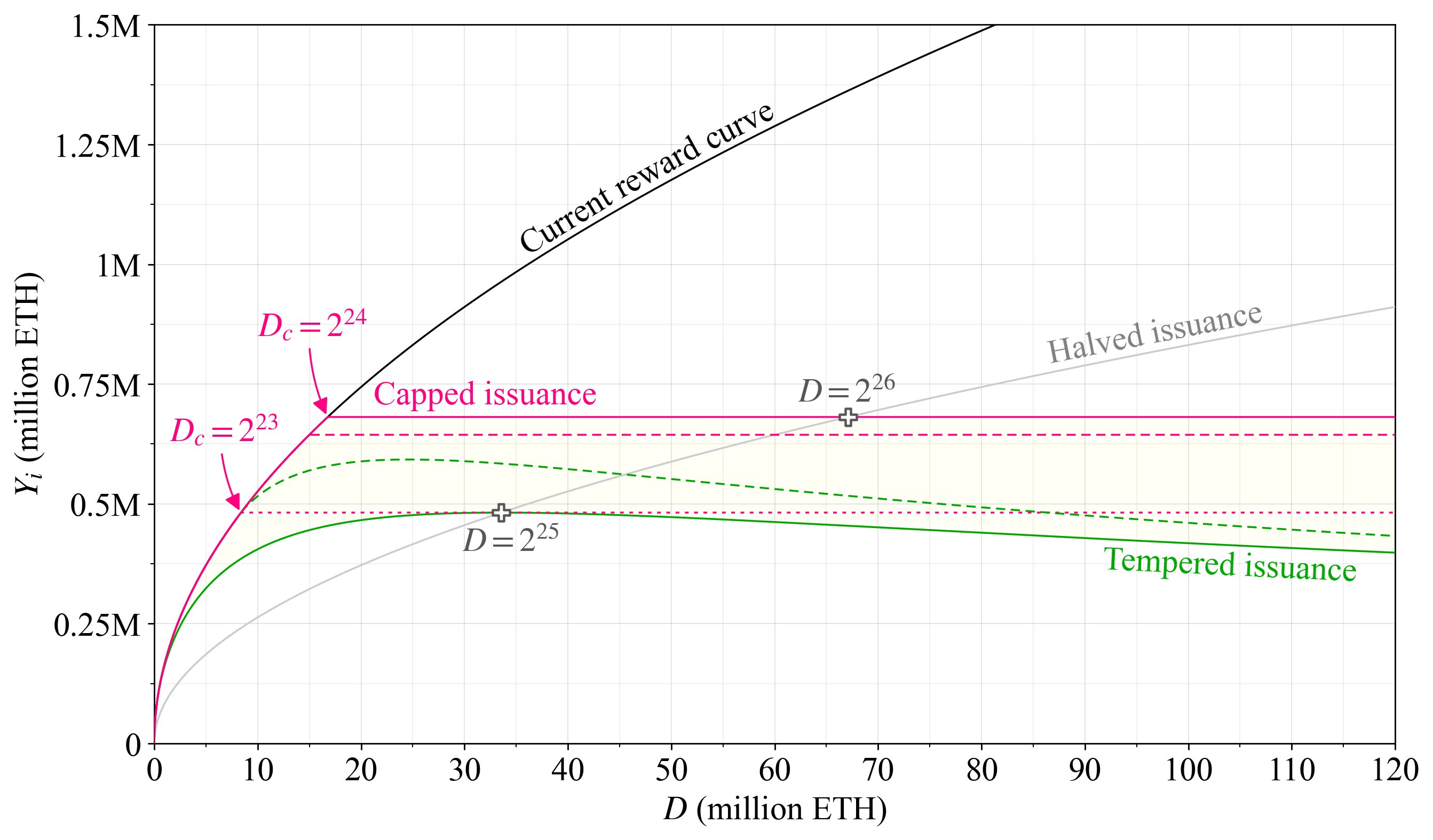
Figure 2. A reasonable issuance range in yellow achieved through a reward curve with tempered issuance (green) or capped issuance (pink).

Reward curve with tempered issuance (green)

The current reward curve in black follows the equation for issuance yield y_i = cF/\sqrt{D}, with the constant c\approx2.6 and the base reward factor set to F=64. Yearly issuance is always Y_i=y_iD. The reward curve with tempered issuance in green is created by division with 1+D/k, thus:

y_i = \frac{cF}{\sqrt{D}(1+D/k)},

with k set to 2^{25}. The variable k defines participation at peak issuance, which also becomes the point where issuance is halved, indicated by the lower cross at around 33.6M ETH. The dashed green reward curve makes a small change to the computation, subtracting a fixed constant k_2 from D (minimum 0) when computing the new term. This constant was here set to k_2=2^{23}. The idea is to provide stronger guarantees of a sufficient quantity of stake and thus security. While this is very unlikely to be required, it might still make the governance process of finding an agreement on the change easier. A similar effect can also be achieved by using a reward curve of a higher order.

Reward curve with capped issuance (pink)

In pink are reward curves with capped issuance (shorter write-up here). The cap D_c defines stake participation when issuance diverges from the current reward curve and flatlines. The lowest setting within the sought range is D_c=2^{23} (8.4M ETH) indicated by a dotted curve and the highest is D_c=2^{24} (16.8M ETH) indicated by a full curve. One interesting detail is that Vitalik Buterin’s active validator cap and rotation proposal from March 2021 has the same effect on issuance as when applying D_c=2^{24}. One benefit of this reward curve is thus its long history, potentially being the first serious proposal for tempering the growth in the actively participating stake. The reader might find the comment section on that post interesting, with early thinking on Ethereum’s circulating supply equilibrium, targeting a participation ratio, and variable validator balances. The dashed pink curve corresponds to the viable option of $D_c=15$M ETH. The midpoint, 2^{23}\sqrt{2} might also be interesting (not plotted).

Staking yield and outlook

Figure 3 shows the staking yield y=y_i+y_v, including MEV yield y_v at the current level of 300k ETH of MEV per year, for some of the previously outlined reward curves (retained color and line style). In blue is the same hypothetical future supply curve as in Figure 1. It is intended to illustrate what the supply curve might look like a few years from now, as a way to understand how an equilibrium might form. The faint blue line may then be the supply curve after another few years have passed and the costs associated with staking have fallen even further. The difference in equilibrium yield between the two reward curves will depend on the slope of the supply curve and, as illustrated, may not be that significant, here amounting to 0.5%.

Figure 3. Staking yield from the outlined reward curves, inclusive of MEV of 300k ETH per year. Two hypothetical supply curves are indicated in blue.

Figure 4 instead shows only issuance yield, with no rewards from MEV. If MEV burn (e.g., 1, 2, 3) is successfully implemented, the staking yield could approach these levels. However, MEV burn is at a rather early research stage with no guarantee of success, and some parts of the MEV such as consensus-layer preconfirmations may never be burned. The figure illustrates that the equilibrium staking yield could also decrease due to a continued fall in the supply curve, after another few years have passed. The combined effect brings down the staking yield to 1.76% in this hypothetical scenario, but it is still within 0.5% of the equilibrium yield with the current reward curve.

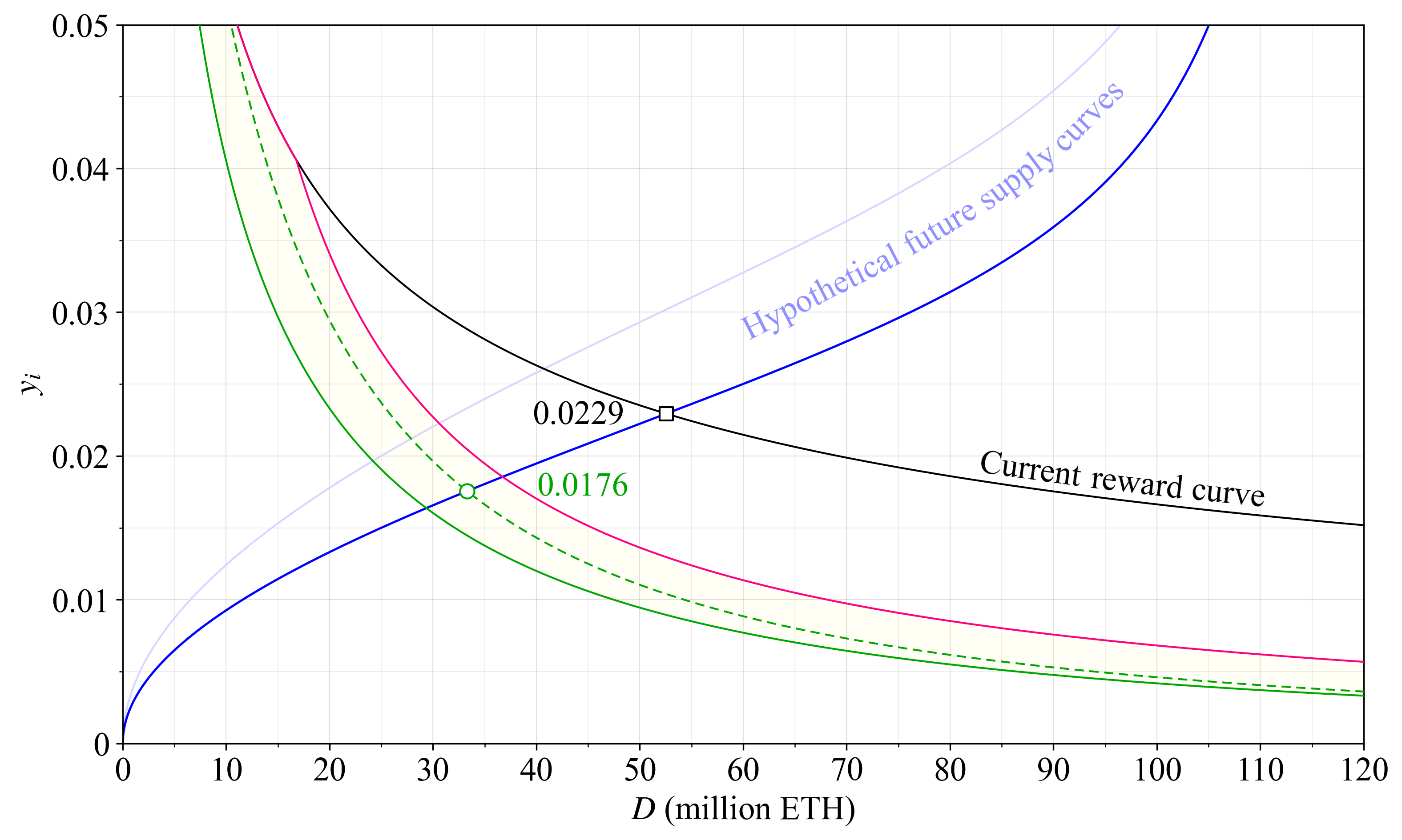
Figure 4. Issuance yield y_i under the outlined reward curves. This is also the staking yield if all MEV has been successfully burned, a scenario that may not materialize. Two hypothetical supply curves are indicated in blue.

It can be noted that the reduced staking yield from MEV burn makes an equilibrium at a desirable quantity of stake rather likely, even if the supply curve continues to fall. Therefore, adopting something close to the dashed green reward curve, followed up by MEV burn a little later, could bring Ethereum to a stage where the quantity of stake is tempered and remains firmly below 60M ETH, likely closer to 30M ETH. This does not mean that this reward curve necessarily must remain in place. But the reward curve should give us plenty of time to continue the debate on the “endgame” issuance policy (see this answer without having to worry about the quantity of stake growing debilitatingly high.

Why not dynamically adjust the yield with a mechanism like EIP-1559 to guarantee some fixed target participation level?

Overview

One common suggestion is that Ethereum should use a mechanism like EIP-1559 to automatically adjust the yield, ensuring that the stake participation is kept at some specific targeted level. Allowing the market to set the issuance yield may seem more neutral, taking away control from developers. Of course, this merely shifts the problem to defining one specific appropriate quantity of stake instead. And what is worse, it constrains Ethereum to purchase an equal amount of security, regardless of its cost. Arguably, there is not one specific appropriate quantity of stake, because the price of the security (the equilibrium issuance level) also matters.

As previously discussed, the marginal increase in security from adding another validator provides diminishing utility as the quantity of stake increases. At some point, the utility loss of excessive issuance becomes greater than the utility gain from more security. Clearly, that point will depend also on the cost of the security. Another concern with a target participation level is that it gives stakers incentives to discouragement attack Ethereum to drive up the issuance, in one version operating as a union. Trying to rectify these flaws will ultimately recreate some form of reward curve, because it is in many ways a more sophisticated solution.

A fixed target participation level is a vertical reward curve with subpar budgeting

When the yield adjusts dynamically to enforce some specific target participation level, the mechanism behaves similar to a vertical reward curve in the long run. Any such mechanism will of course adapt gradually to avoid too big changes in yield from small shifts in the supply curve, but the equilibrium ultimately returns to a point where the supply curve intersects the vertical “dynamic” reward curve. Two such reward curves are illustrated in magenta in Figure 5, one where the target has been set to 30M ETH staked and one at 60M ETH staked. The figure presumes 300k ETH in MEV per year. A regular reward curve “Endgame (3)” presented in another answer is instead shown in purple.

Figure 5. Equilibria under various supply curves in blue when using a fixed target participation level (magenta), a reward curve with cut issuance (purple), or the current reward curve (black). Green circles represent desirable outcomes, red crosses undesirable outcomes, and yellow triangles are outcomes somwehere in between. As captured by the red crosses, a fixed target does not facilitate proper budgeting.

Three hypothetical supply curves are shown in blue, intended to illustrate what the outcome would be under vastly different scenarios. With a 30M target under a high supply curve, an equilibrium forms at a 2.87% staking yield; a desirable outcome under the presence of MEV as marked by a green circle. Under the outlined medium supply curve, an equilibrium forms at 1.87% instead. This might be perceived as slightly problematic because MEV will constitute 53.5% of the total staking rewards. As a result, block proposals bring home around 59.3% of all rewards under the current consensus specification, and so the equilibrium is marked by a yellow triangle to indicate a medium outcome. Yet, it is rather close to being classified as a green circle in my view. The equilibrium under the low supply curve at a 0.5% staking yield is marked by a red cross to indicate undesirability. This equilibrium happens under a negative issuance yield since the MEV yield is 1%. Non-pooled stakers (e.g., most solo stakers) must then lose money each epoch in the hope of eventually being assigned to propose a block.

With a 60M target under the high supply curve, an equilibrium forms at a 4.6% staking yield. This is very undesirable. Ethereum would in this scenario issue 2.45M ETH per year when the equilibrium issuance of 0.56M ETH at 30M ETH would be sufficient. The downside of course is the unnecessary costs that Ethereum is subjecting its users to. For the users, this manifests as being coerced into taking on some of those costs as a staker, or otherwis see their savings eroded by dilution. The equilibrium for the medium supply curve is also undesirable for the same reason. The equilibrium at the low supply curve however seems acceptable, at a staking yield of 1.11%. The MEV is a bit high at 45% of the rewards, and indeed the proposer gets 51.8% of the expected staking yield. Yet this seems acceptable in order to keep the quantity of stake from growing too high under a low supply curve, where 60M ETH is already undesirably high.

The problem with a dynamic reward curve and a specific target is that the associated vertical shape may lead to undesirable staking equilibria. The reader will note that by using the purple reward curve denoted as “Endgame (3)”, an acceptable equilibrium is reached under all three supply curves, as marked by green circles. If the supply curve is higher, an equilibrium with a low quantity of stake is attained, ensuring that the costs to Ethereum’s users do not grow too large. If the supply curve is lower, the quantity of stake is allowed to grow to ensure that a reasonable issuance yield is provided to stakers. This also enables Ethereum to ensure a viable composition of the staking set.

The future level of the supply curve will always be unknown, and the reward curve (the demand curve) must therefore be designed to produce acceptable outcomes in any reasonable scenario. A desirable reward curve can in a way be understood as the expansion path that optimizes between yield and stake participation across potential supply curves, as outlined in a subsequent answer. The current reward curve is shown in black and will as indicated produce excessive issuance (costs to users), while also leading to an undesirably high quantity of stake under lower supply curves.

Ethereum is currently researching MEV burn. This would alleviate some of the concerns with particular equilibria leading to excessive proportions of MEV. The outcome under full MEV burn is shown in Figure 6.

Figure 6. Equilibria under MEV burn for various supply curves in blue when using a fixed target participation level (magenta), a reward curve with cut issuance (purple), or the current reward curve (black). Green circles represent desirable outcomes, red crosses undesirable outcomes, and yellow triangles are outcomes somwehere in between.

Equilibria at lower staking yields when 30M ETH is staked are less problematic if there is no MEV. For example, non-pooled stakers would receive positive rewards each epoch. The equilibrium under the low supply curve is still marked by a yellow triangle. It could be fair to mark it by a green circle, but in my opinion, we might wish to let the quantity of stake expand somewhat under these supply curves. This gives a higher equilibrium yield and will give better guarantees of a viable composition of the staking set. One way to understand it is that the reward curve helps absorbs all delegating stakers with a low reservation yield to ensure that the yield remains viable for solo staking.

Figure 7 below plots the total yearly rewards (corresponding here also to total issuance, since MEV burn is in place in this example). The excessively high issuance under high supply curves and a fixed target of 60M ETH is very problematic. Likewise concerning the high issuance under low supply curves with the current reward curve. Note that the really problematic outcomes for the current reward curve instead happens under low supply curves, because it is designed to increase issuance as the quantity of stake increases.

Figure 7. Yearly issuance under MEV burn for various supply curves in blue when using a fixed target participation level (magenta), a reward curve with cut issuance (purple), or the current reward curve (black). Green circles represent desirable outcomes, red crosses undesirable outcomes, and yellow triangles are outcomes somwehere in between. A fixed target of 60M ETH (magenta) will lead to excessive issuance if the supply curve is higher.

A fixed target participation level may incite stakers to attack Ethereum

The previous section established the downside of not attaching a proper budgeting mechanism to Ethereum’s security expenditures. It may lead to Ethereum overpaying for security, or paying so little that solo stakers needlessly are driven out. Some may consider concerns around solo staking overblown, and feel that the benefit of a specific target outweighs, because Ethereum will at least have some specific participation level that has been deemed appropriate by the community. The issue with a fixed target is however a little deeper. Stakers need to come to consensus under listener–speaker fault equivalence, something that opens up avenues for discouragement attacks. The protocol cannot ascertain who is at fault for a failed consensus message delivery. An attacker can therefore act maliciously against honest consensus participants to deprive them of rewards, subsequently profiting as they leave and the staking yield increases. There exists various avenues even for minority discouragement attacks at the present.

With a fixed target participation level that adapts relatively quickly, the “p_i-elasticity” becomes infinite. The incentives for discouragement attacks are then maximized; less stake must leave to drive up the yield. A related concept is cartelization attacks, consisting of SSPs working together to try to reduce quantity staked, potentially also among themselves. When issuance increases with a reduction in quantity staked (p_i>1), all stakers could try to agree to reduce their stake, and everyone would be better off (as long as new entrants are kept out or discouraged). This framing can provide a suitable backdrop for convincing the social layer to not interfere when a staking cartel tries to inhibit Ethereum’s permissionlessness, utilizing discouragement attacks.

The importance of discouragement attacks should not be overblown, but it is unnecessary to open up for them when safer designs so easily can be achieved. It is particularly striking that under the strict target, attacking the consensus through censorship can generate what is essentially an infinite-money glitch without breaking validity.

Rectifying the outlined flaws recreates a subpar reward curve

To protect against stakers turning the consensus mechanism into a money-printing machine, the protocol might of course impose some maximum yield beyond which no further increases are deemed necessary (besides relying on the social layer and the threat of intervention). For good measure, the issuance policy may also define a floor, so that stakers always receive some yield, ensuring a viable composition of the staking set. Figure 8 plots this new hypothetical updated fixed target reward curve (once again ignoring the time component). The ceiling was set to 5% and the floor to 0.25%.

Figure 8. A fixed target participation level with upper and lower limits, attempting to rectify some issues of the design shown in Figures 5-7. However, a reward curve remains the better solution.

The mechanism now prevents the infinite-money glitch, and gives stakers at least some guaranteed yield. However, it arguably remains flawed, with improper budgeting. The incentives for discouragement attacks and cartelization attacks are still unnecessarily pronounced in the vertical part of the curve. The fixed floor and ceiling should instead have the smooth characteristics of a reward curve, gradually increasing or decreasing as the utility function changes.

The outlined flaws do not mean that there is no value in a dynamic approach; it is possible to combine it with a reward curve. The idea would be to allow the reward curve to drift/bend at longer time scales, ultimately being influenced by a separate target reward curve. Such a “time–quantity policy” is explored in the answer on the staking economics endgame.

How will a reduction in issuance affect the composition of the staking set?

Overview

This depends on how sensitive relevant groups such as solo stakers and delegating stakers are to low staking yields and high variability. One concern is unfavorable economies of scale for solo stakers at low yields. At the same time, the delegating staker subjects itself to unique risks when trusting a third party with its ETH, and may for this reason also be hesitant to stake if the yield goes too low. There is furthermore a dynamic at play wherein delegated staking becomes relatively more favorable as the quantity of stake grows. There is thus a multitude of conflicting economic forces to consider. One way to approach this complex subject is by comparing distributions that attempt to capture the willingness to stake at different yields among solo stakers and delegating stakers, as shown, for example, in Figure 11 below.

It is important to understand the probabilistic nature of issuance policy, and that the design ultimately tries to optimize outcomes under any scenario (e.g., a lower or higher supply curve). As outlined in another answer, a suitable reward curve can in this context be understood as the expansion path across potential supply curves that optimally balances trade-offs. One of these trade-offs is the equilibrium composition of the staking set. With this viewpoint and in light of potential concerns, an equilibrium at 30M ETH can be desirable, but still not enforced by economic capping. Under a particularly low supply curve, the quantity of stake can be allowed to expand. The composition of the staking set must thus ultimately be analyzed and optimized for across two dimensions, both issuance level and quantity of stake.

Variability for solo stakers

If issuance is moderated, a larger part of rewards will stem from REV, and the relative variability in staking rewards will therefore increase. This affects solo stakers negatively since they cannot effortlessly rely on pooling for smoothing out variability. A review of how variability affects the solo staker is offered in a previous write-up on properties of issuance level. It seems reasonable to assume that stakers may be more more sensitive to variance at lower staking yields—the relative variability matters. This of course certainly holds true under an equilibrium where the issuance yield is negative but the staking yield (which includes REV) is positive—for example when instituting economic capping (1, 2). Solo stakers that do not pool their execution layer rewards will then need to lose ETH each epoch in the hope of being assigned to propose a block. Since MEV yield is shared among stakers, it rises with a lower quantity of stake, and such an equilibrium therefore becomes increasingly more likely the lower the economic cap is set, because the MEV yield can then still be a sufficient incentive on its own. Relative variability is one of the reasons for pursuing the more moderate reward curves discussed in a previous answer before MEV burn is in place. This does not mean that a low economic cap will be enforced afterward, merely that it is much more feasible once MEV burn is in place.

Equilibrium yield and the proportion of solo stakers

Ethereum wants to retain solo stakers, at least when measured as a proportion of all stakers. The anticipated outcome of a reduction in issuance level is that less ETH will be staked by both delegating and solo stakers, relative to the outcome when issuance is not reduced (1, 2). A concern is if there might be a staking yield below which solo stakers in particular would drop off due to, e.g., the relatively higher fixed costs associated with solo staking.

Take for example Figure 3 as a starting point. It is not clear whether the proportion of solo stakers is lower at a hypothetical equilibrium of around 36M ETH staked and a staking yield of 2.44% (green dashed reward curve with tempered issuance) than at around 50M ETH staked and a staking yield of 2.94% (black current reward curve). If solo stakers leave en masse below a yield of 2.6%, then a staking yield of 2.44% at 36M ETH staked will give a lower proportion than when the yield is 2.94% at 50M ETH staked. This is of course something to take seriously. Economies of scale are hard to design away in a decentralized blockchain.

There are however also some arguments as to why a more restrictive reward curve could give a higher or at least similar proportion of solo stakers:

Dominant SSPs have better economies of scale at higher quantities staked, increasing their cost advantage over solo stakers.
Likewise, the positive network externality of the money function grows with quantity staked, and with it the competitive advantage of dominant LST-issuing SSPs.
Furthermore, the principal–agent problem associated with an LST may seem less risky if everyone else also uses the LST, with the expectation that the social layer will waver on its commitment to the intended consensus process in the event of a failure.
Risks could very well price out delegating stakers earlier than solo stakers as the yield falls. For example, if a large enough subset of potential delegators believe that there is a 1% risk of failure over a year for the LST they wish to hold, then favorable economies of scale or liquidity can be insufficient as a competitive edge. Self-custody is undeniably important to a relevant proportion of ETH token holders; this factor should not be overlooked when evaluating the staking supply side.
On a similar theme, if the yield becomes negative, there is still an altruistic motive for solo staking. The delegating staker will either need to take on a loss or face adverse selection. An SSP that subsidizes delegators will do so under the expectation of future profits, which may be attained by monopolizing some critical function, or worse, by attacking the consensus. An SSP profiting from restaking could just as well profit using non-staked ETH.
Token holders with enough ETH and the technical ability to solo stake are not necessarily abundant, implying a soft upper bound on the solo staked quantity. It can be argued that if this pool is more or less depleted, then relatively few of the new stakers will be solo stakers as the supply curve falls and D increases under the current policy. Still, concerning this particular argument, it should be remembered that if the yield is reduced substantially to halt the increase in D, there is no guarantee of retaining a larger proportion of solo stakers in the long run. This ultimately depends on the finer-grained distribution of reservation yields among them, as explored in the next subsection.

Issuance policy should be focused on long-term objectives and not rely on short-term remedies. This also relates to the presently rather valuable solo staking airdrops, if they can be expected to cease. Yet, Ethereum’s evolving consensus mechanism may look different in ten years, with different requirements for staking anyway—there may even be different classes of validators (1, 2)—so circumstances of the present and in the near-term future cannot be completely ignored. For example, it must be acknowledged that if the yield falls, the impact of any solo-staking airdrops will multiply. As an example, if their expected value is 1% per year, and the staking yield falls from 4% to 1%, then airdrops will go from giving solo stakers a 25 % higher revenue than the delegating staker to giving a 100% higher revenue.

An additional nuance can also be added to the fourth bullet point: some solo stakers stake quite a bit more than 32 ETH, and these may be more resilient to low yields. Finally note that solo stakers who do not own their hardware may still enjoy some external economies of scale; home stakers on the contrary are directly affected by hardware costs.

At a fundamental level, the conjecture is that the relative distribution of reservation yields may differ between different classes of stakers. This then leads to different proportions of solo stakers under different issuance policies. But whether one policy is better than the other in this respect cannot be ascertained and may also vary over the forthcoming decade.

Relative distribution of reservation yields

This subsection will explain the conjecture from the previous paragraph by visualizing some hypothetical distributions of reservation yields among different classes of stakers. Naturally, such distributions emerge from some fundamental functions capturing the willingness to supply stake, which ultimately depends on the composition of those seeking exposure to the ETH asset and how they value various costs associated with staking. I will present such models at a later date. These visualizations will simply illustrate what the distributions might look like based on the ideas presented in the previous subsection, without quantifying the actual underlying economic forces.

The notion of a “reservation yield” is lent from labor economics, in which reservation wages influence the quantity of supplied labor across wage (the labor supply curve). Staking economics and labor economics have some similarities; after all, staking is work done to maintain the consensus process, and stakers—just as workers—can under certain circumstances cartelize (i.e., a labor union/cartelization attack) as discussed in a previous answer. The laborer’s valuation of their leisure time to some extent then corresponds to the premium that the token holder attaches to non-staked ETH. It should however be mentioned that the “reservation yield” here applies to a “prospective” token holder. The purpose is to capture the specific yield at which some token would be staked, but it must be recognized that the actual token holder might change due to changing circumstances.

A specified reservation yield is assumed to apply under the equilibrium formed also when accounting for other stakers’ reservation yields, and stake will not switch staking modality across staking yield. Also note that the reservation yield represents what the staking yield must be, and is not a staker’s profit, because there are also costs/fees. The example is intended to capture what the distributions might hypothetically look like a few years from now, assuming that a functioning MEV burn is in place and that airdrops to solo stakers unfortunately have become less ubiquitous.

Illustrating hypothetical distributions of reservation yields

The dotted line in Figure 9 shows a hypothetical distribution of reservation yields for solo stakers, with staking yield on the x-axis. Presumably, not many stakers have a zero or negative reservation yield. A tiny few might be inclined to stake even if there are no direct monetary incentives provided by the consensus mechanism (a staking yield of 0), perhaps to defend or attack the network. But these incentives are not something that Ethereum would like to rely on. As the staking yield rises, each marginal increase brings in a larger subset of ETH token holders as solo stakers. The pool of prospective solo stakers then gradually depletes as the overall staking participation rate increases, the curve peaks (here at around 2%), and an increase in yield will ultimately not bring in many new stakers.

Figure 9. Hypothetical distribution of reservation yields among solo stakers.

Figure 10 instead shows with a dashed line what the distribution of reservation yields among prospective delegating stakers may look like. The distribution might generally have a more positive skew. The idea is (a little simplified) that the last quartile of stakers favor liquidity and might not have the technical ability to solo stake, whereas favorable economies of scale bring a sharper increase at lower yields. The previously illustrated hypothetical distribution of solo stakers is also included in the plot, but they are relatively fewer, so it is hard to compare the shapes.

Figure 10. Hypothetical distribution of reservation yields among delegating stakers (dashed line). The distribution for solo stakers from the previous Figure 9 is also included (dotted line).

To make comparisons easier, Figure 11 instead shows both distributions normalized to represent an equal share of all ETH. Still, remember that these curves are just an attempt to illustrate the ideas presented in the previous subsection, and as such are hypothetical. But this caveat might on the other hand always be applicable, even under more deliberate models. The relative comparison of distributions captures the notion that a smaller proportion of delegating stakers would be willing to stake at a negative yield, given the potential for adverse selection and less clear altruistic motive. But then the distribution might shoot up quicker than for solo stakers as the yield becomes positive, due to the favorable economies of scale of delegated staking. As the yield increases further, solo staking comes into play, but then dwindles, because the last quantile of stakers are unwilling to give up liquidity or technically unable to solo stake. The proportion of solo stakers might thus vary intermittently.

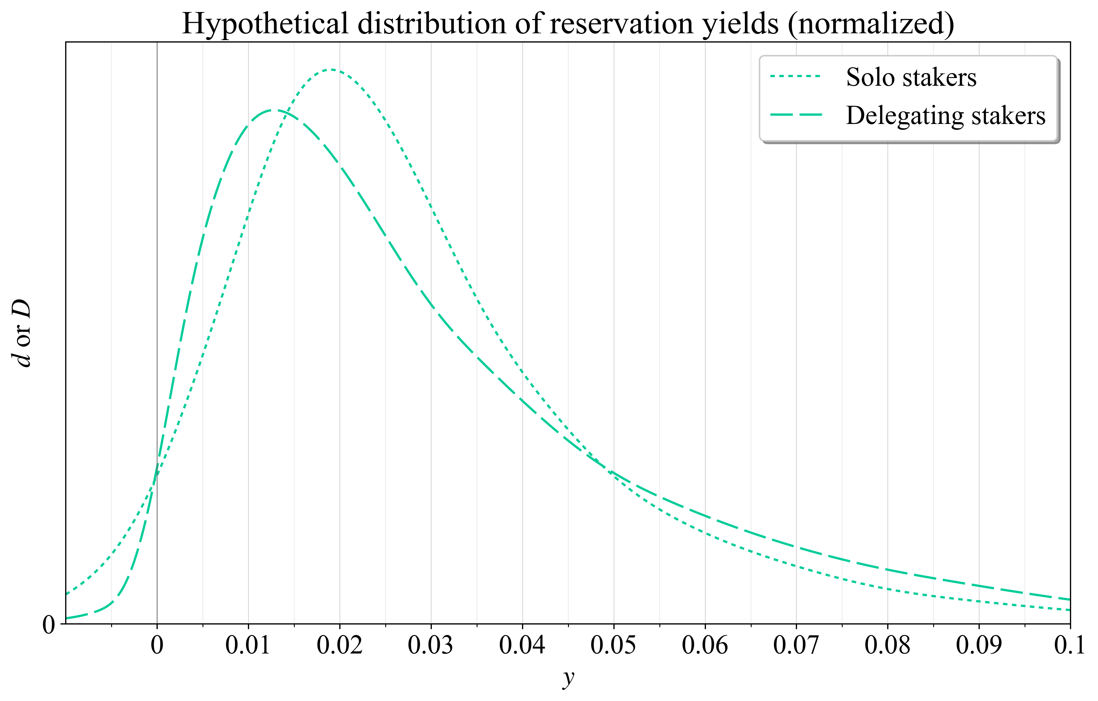
Figure 11. Hypothetical distribution of reservation yields for solo stakers and delegating stakers, normalized to represent an equal share of all ETH.

Having reviewed two hypothetical distributions, it is now time to review how the proportion of solo stakers evolves across staking yield under them. The cumulative distributions are then computed, seeing that a staker will stake at any yield above their reservation yield. These are shown in Figure 12. A way to understand these plots is that the initial distribution is treated as a probability density function (PDF), and its corresponding cumulative distribution function (CDF) then is computed.

Figure 12. Hypothetical cumulative distribution of reservation yields for solo stakers (dotted), delegating stakers (dashed), and in aggregate (full).

The proportion of solo stakers is simply the solo staking CDF divided by the aggregate CDF, as shown in Figure 13. It is not asserted here that this particular outcome would materialize, but it is illustrative of the kind of concepts present in the debate. There is a higher proportion of solo stakers at negative yields, but then some valley at low staking yields due to economies of scale. It can emerge, e.g., if the delegating stakers’ assigned risk premium is more dispersed than the fixed cost structure of solo stakers. Proponents of a higher issuance level would suggest that this valley exists and is pronounced (when removing solo-staking airdrops), but there are many nuances beyond economies of scale to consider, as previously outlined. In any case, it is not clear that the effect would necessarily be that significant.

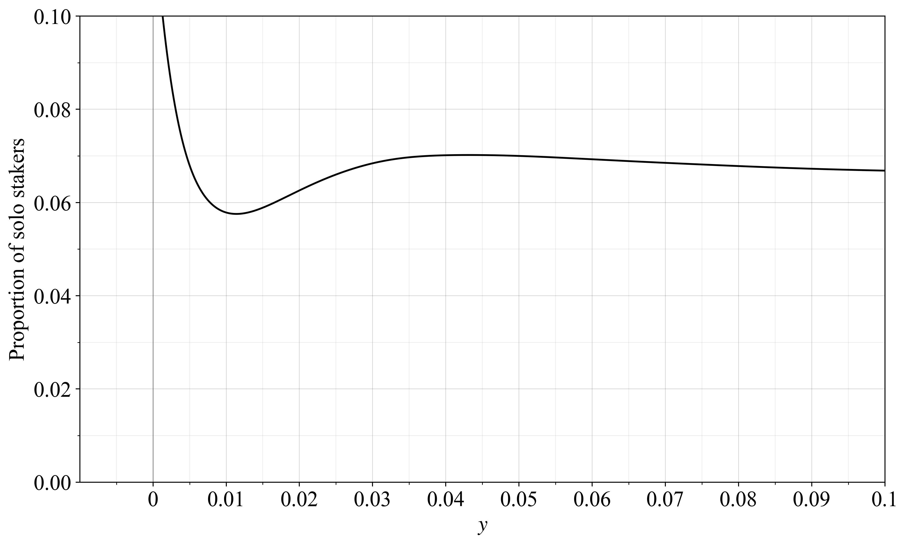
Figure 13. Hypothetical proportion of solo stakers across staking yield.

Since each point of the supply curve represents the reservation yield of the marginal staker, the cumulative distribution of reservation yields actually corresponds to the supply curve. To make this clear, simply flip the axes of Figure 12 to have yield on the y-axis and stake on the x-axis. The supply curve then emerges in its more common presentation, as shown in blue in Figure 14. Two reward curves are included with no MEV—the current reward curve in black and the moderate reward curve with capped issuance at D_c= 15M ETH from a previous answer. Two hypothetical equilibria are indicated by squares, at the intersection of the aggregate supply curve and these reward curves. The participation ratio of solo stakers and delegating stakers are simply found along the horizontal line extending from the equilibrium, at the point where this line intersects the associated set supply curve (circles).

Figure 14. Cumulative distribution of reservation yields, here illustrated as a supply curve in blue, with flipped axes from Figure 12. Set supply curves for delegating stakers and solo stakers are also indicated. Stake participation of each class (circles) are found at the horizontal line extending from the equilibrium (squares).

Note that the hypothetical distributions here presented only give one specific supply curve. Under another lower supply curve, the distributions would presumably be compressed such that many features, e.g., the transition to favoring delegated staking, emerge at a lower yield. I have been working for quite some time on a complex probabilistic model trying to unify these considerations, and hope to present it in a while. This topic is certain to receive further attention also from other researchers (e.g., 1, 2, 3).

Equilibrium yield and the broader composition of the staking set

The relationship between issuance level and diversity in SSPs also entails a trade-off between economies of scale and factors such as the positive network externality of the money function. Offering a positive yield beyond 30M ETH is helpful for alleviating concerns that a major SSP with a structural advantage such as a centralized exchange (CEX)—perhaps leveraging some hypothetical staked ETF—can push up their proportion of the stake to critical levels. At the same time, the risks of centralization around such entities should not be disproportionately emphasized over other risk scenarios. There are already today SSPs attaining critical proportions of the stake by leveraging network externalities onchain, ostensibly foregoing profits in the pursuit of monopolization. This type of structural advantage could also grow with higher issuance, and stifling that before native ETH possibly is in the minority relative to one LST must be considered as a net positive to the community. When weighing these trade-offs, an issuance level that invariably forces any outcome—whether a very low or very high quantity staked—does not seem desirable.

Each SSP, reaching for a specific market segment, incurs unique costs besides the cost of running staking nodes, with a wide variety ranging from compliance to software. Indeed, CEXes have somewhat of a local monopoly on their customers-as-delegators, and the opportunity cost of keeping fees competitive with any onchain option is presumably so high that it does not represent the profit-maximizing strategy. What is clear is that competition for delegated stake will unfold across diverse market segments, and perfect competition is not a reasonable assumption. If the cost of operating a node is not prohibitively high relative to the income that the SSP can make from running it, then variety in preferences and circumstances between delegators will take a central role in shaping the composition of the staking set. The concern is therefore only valid with a yield that goes close to 0 or negative at a low quantity of stake. No SSP can reasonably outcompete all others at an equilibrium staking yield of, e.g., 2% at 30M ETH staked.

What is the endgame issuance policy?

Overview

Certain parts of the endgame have a rather broad agreement. Firstly, Ethereum should transition to using d (referred to in this text as the deposit ratio or stake participation ratio) in the equation for the reward curve instead of D (deposit size or quantity staked). This can simply be done (1, 2) by swapping out D for d in the equation for the reward curve, and normalizing by including the circulating supply at the time of the swap, once the circulating supply begins to be tracked at the consensus layer. The main reason for this transition is that the long-run staking equilibrium under reward curves that adapt to D instead of d is ultimately also influenced by the circulating supply equilibrium, since the circulating supply will drift to balance supply, demand, and protocol income.

Secondly, Ethereum should pursue MEV burn. As explained in the previous answers (1, 2), this will reduce relative variability and is a prerequisite for being able to reduce the staking yield substantially without causing too much concern for non-pooled stakers. As the answer soon turns to reduced issuance, it must be remembered that there is no direct financial motive for staking if the endogenous staking yield (MEV + issuance + airdrops) is negative. An equilibrium at negative issuance attracting a sufficiently large quantity of stake should thus still involve a positive expected endogenous yield. One concern is that the variability in MEV then involves non-pooled stakers taking on small losses each epoch while they wait for being assigned to special duties (note that variability in airdrops are not resolved by pooling). But there are many other reasons for MEV burn as well, as explored by Francesco, Justin, as well as Mike, Toni, and Justin.

The endgame when it comes to issuance level is currently a subject of debate but does indeed by all accounts involve an issuance reduction. The options can roughly be divided into five different categories:

Do nothing; an alternative that must always be part of the conversation, but which is becoming increasingly less attractive assuming that staking costs continue to fall and the quantity of stake increases further.
Temper issuance; but to a level that is perfectly sufficient also under the presence of MEV.
Cut issuance; an option situated in between (2) and (4). Does not institute an economic capping, but makes a high quantity of stake incredibly unlikely by lowering the yield substantially.
Economic capping, by letting the staking yield go to negative infinity at some desirable quantity of stake.
A time–quantity policy; where the reward curve is allowed to slowly alter/bend in response to changes in the supply curve.

Among these options, (2) is becoming increasingly desirable at this point in my view. There is then a sliding scale from (3) to (4), where stricter reward curves are advantageous due to their ability to offer guarantees on the quantity of stake, while some restrictive settings at the same time also require more deliberations. There can be merits to an economic cap (4), ideally then after MEV burn, but in my view not at a too low quantity of stake. Some examples will be illustrated. Category (5) has not yet received much study and will be presented a little deeper. The answer will now briefly review the philosophical underpinnings of the optimization problem, and then take a closer look at each of the five categories.

Philosophical underpinnings of the optimization problem

The reward curve is in essence an attempt to optimize between all known trade-offs (long-run and short-run economic security, low costs, a viable composition of the staking set, reward variability, etc.), ensuring a utility-maximizing equilibrium under any supply curve. One way to understand the issue is thus that each hypothetical supply curve (low as well as high) has one optimal equilibrium, and the reward curve should intersect each supply curve at this point.

In economics, an expansion path connects optimal input combinations across output level, and an income expansion path selects the optimal consumption bundles across income. A suitable reward curve is the expansion path that optimizes all known trade-offs associated with high/low yield and stake participation across potential supply curves. Figures 5-8 in a previous answer illustrated the concept under three supply curves at different levels, where an optimal equilibrium could be found under all three using a reward curve from endgame (3).

As framed by Vitalik in a similar context: if a reward curve is designed such that some specific equilibrium is made possible, then that equilibrium should first have been deemed acceptable. In particular, it should ideally be the optimal equilibrium for the prevailing supply curve. But it must then also be noted that not only the level, but also the shape of the supply curve will matter. The reason is that the shape will influence which alternatives a specific equilibrium point can be substituted for when optimizing. There is a difference between the almost horizontal supply curve between 30M and 120M ETH in figures by Caspar and Ansgar, and the supply curves in this post that slope almost vertically upwards towards 120M ETH. In the former case, setting a negative yield at 30M ETH will seem like a more natural solution, because an economic cap at a low quantity of stake might not matter to solo stakers anyway, regardless of if the supply curve is lower or higher.

1. Do nothing

This option remains valid while the quantity of stake remains reasonably close to 30M ETH (1/4 of the stake), previously discussed as a potential limit. There is a switching barrier associated with changing the issuance policy of a decentralized blockchain. The potential for discontent is higher if the switch takes place too close to previously discussed limits. But as mentioned in another answer, it seems reasonable to assume that the current quantity of stake of 32M ETH will not hold in the long run, as staking costs (broadly defined) fall. A threshold that would fit neatly with the notion of operating on powers of two is 2^{25} ETH, corresponding to 33.6M ETH. Once this threshold is exceeded (or on the path of being exceeded) when doing nothing, then doing something seems like a better option to me.

Excessive incentives for staking, beyond what is necessary for security, can unfortunately over time turn into perverse subsidies. In a scenario where the application layer is built around excessive staking yield, the Ethereum economy will arguably not have proper trustless foundations, as previously discussed.

One thing to keep track of before deciding to “not do nothing”, and to “do something”, is the progress of MEV burn. A reduction in issuance should not take place at the same hard fork as when incorporating MEV burn. If MEV burn is very close to being ready, then this can be accounted for under certain circumstances. But MEV burn is still at an early research stage. One path is therefore to shortly institute a moderate reduction in issuance, a year or two before MEV burn, and then let MEV burn make another dent in the staking yield.

2. Temper issuance

This option is presented in a previous answer. In summary, it represents a “safe” issuance reduction that will not increase relative variability too much for non-pooled stakers, providing a relevant staking yield for stakers across the full range. The option provides a sufficiently big reduction in issuance to make the associated governance process worth it—and small enough to make that process potentially easier. The option will still substantially temper the growth in the quantity of stake. Together with MEV burn, it can reasonably constitute an endgame issuance policy, in the sense that the quantity of stake remains close to 30M ETH and firmly below 60M ETH. However, this does not mean that (2) necessarily must be an endgame. Reducing the issuance even further at higher quantities of stake as in (3) and (4) will after MEV burn seem like a reasonable option. However, proceeding further than (2), for example to (4), would then need to be a separate discussion. There is a simple “on-switch” that could be used for such a transition, as discussed in the associated subsection.

3. Cut issuance

I refer here to the option situated in between economic capping and tempered issuance as “cut issuance”. The limits of this category are a bit diffuse, but it attempts to capture reward curves that are intended potentially for an Ethereum with MEV burn, that still does not pursue economic capping. Figure 15 shows three examples, with the pink curve close to category (2) and the violet reward curve bordering on category (4). The current reward curve is shown in black and the limits of the capped issuance curves that are part of (2) are indicated in grey for reference.

Figure 15. Three reward curves that cut issuance substantially, without definitely capping stake participation.

The pink and purple curves rely on the same strategy of making as small adjustments as possible to the current protocol, as previously introduced. The pink curve has the equation

y_i = \frac{cF}{\sqrt{D}+(D/k)^2}

with k=2^{19}. The purple curve has the equation

y_i = \frac{cF}{\sqrt{D}(1+(D/k)^2)}

with k=38\times10^6. All reward curves in the figure have F=64. One idea behind these sorts of reward curves that would have a positive issuance yield across the full range also after MEV burn has been instituted is to provide guarantees to solo stakers that the issuance yield will always stay positive. Of course, the staking yield (issuance + MEV) should intuitively always stay positive, since there is no point in staking unless the endogenous yield is positive. But the guarantees here pertain to issuance yield, meaning that solo stakers might always be able to enjoy a positive yield on a more regular basis (even without being assigned as proposer from time to time) under circumstances where some MEV still remains (due to, e.g., a partial MEV burn or consensus layer preconfirmations).

The violet curve subtracts (D/k_2)^2 from the purple curve, with k_2=9\times10^8. The effect is that the staking yield gradually turns negative, without ever going to negative infinity. This is a more restrained way to use negative yields. In reality the effects would be very similar. Some hypothetical benefits are that the equilibrium cannot happen at a point where the yield falls very sharply at the limit (influenced by a high MEV scenario) and that stakers will have better guarantees of not encountering a double-digit negative yield (which of course should not happen anyway). A downside is that there are no hard guarantees of capping the quantity of stake. Figure 16 shows the staking yield (inclusive of 300k ETH in execution layer rewards per year) and Figure 17 shows the issuance yield (no MEV).

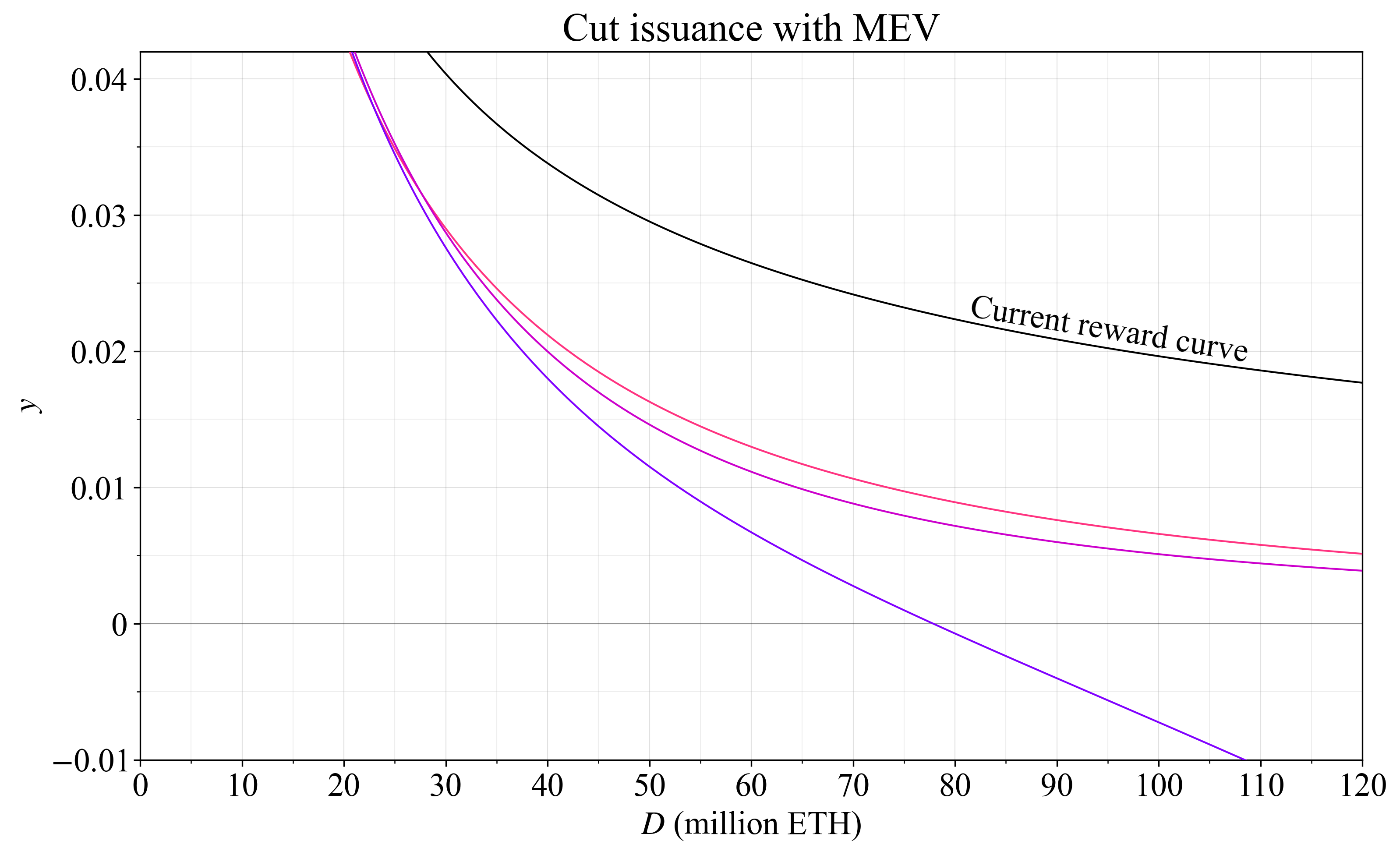
Figure 16. Staking yield under three reward curves that cut issuance.

Figure 17. Issuance yield under three reward curves that cut issuance.

4. Economic capping

Economic capping was introduced by Vitalik as a way to guarantee that the quantity of stake does not grow beyond some set limit. A more extensive write-up on economic capping was recently provided by Caspar and Ansgar, including the notion of applying (4) after (2). Vitalik’s reward curve can be generalized to

y_i = \frac{cF}{\sqrt{D}} - \frac{cF_c}{\sqrt{l-D}},

here adapting the equation to a format that easily can be incorporated directly into the protocol spec. The first term is the current reward curve, and the second term is subtracted from it. Since the second term will go to infinity when the limit l=D, the staking yield will go to negative infinity at that point, capping the quantity of stake. Vitalik used l=2^{25}. The variable F_c shapes the magnitude of the reduction leading up to the cap, and was set to 32 in Vitalik’s curve (implied by 0.5\times64 in his equation). Figures 18-21 show this reward curve in red.

The first term of Vitalik’s equation can be swapped out for some other reward curve, as desired, to allow Ethereum to produce a desirable issuance in the critical region around 20M-40M ETH where an equilibrium is the most desirable. Using the purple curve from the previous subsection gives the equation

y_i = \frac{cF}{\sqrt{D}(1+(D/k)^2)} - \frac{cF_c}{\sqrt{l-D}}.

Figure 18 shows reward curves produced from this equation with a cap set at l= 60M ETH (1/2 of the stake; orange), l= 80M ETH (2/3 of the stake; yellow) and l= 90M ETH (3/4 of the stake; lime). All curves have k=2^{26} and F_c=2^4.

Figure 18. Issuance under reward curves that institute economic capping. The red reward curve is Vitalik’s previous proposal, and the other three reward curves cap the deposit size at 60M ETH, 80M ETH and 90M ETH respectively.

Figure 19 shows the staking yield (inclusive of 300k ETH in MEV per year) and Figure 20 shows the issuance yield (no MEV).

Figure 19. Staking yield including 300k ETH in MEV under reward curves that institute economic capping. The red reward curve is Vitalik’s previous proposal, and the other three reward curves cap the deposit size at 60M ETH, 80M ETH and 90M ETH respectively.

Figure 20. Issuance yield under reward curves that institute economic capping. The red reward curve is Vitalik’s previous proposal, and the other three reward curves cap the deposit size at 60M ETH, 80M ETH and 90M ETH respectively.

A cap at a low quantity of stake under MEV is not desirable, due to among other things the high relative variability, as discussed in previous answers (1, 2). In my view, if Ethereum is to pursue economic capping, then reward curves that institute the cap at or above 60M ETH seem more promising, even after MEV burn. This will allow the quantity of stake to expand somewhat under particularly low supply curves. Yet, having a cap offers an ultimate guarantee and this can be very useful from a macro perspective. At some higher stake participation, the expansion path should therefore arguably venture into negative issuance yields (which will still lead to a positive endogenous staking yield under equilibrium), and this expansion path could then ultimately reach such a low negative territory that it can only be reached with an economic cap. In simpler terms, the negative aspects of stake participation growing very large are worse than the negative aspects of having a very low issuance yield.

A beneficial feature of the presented equation system is that the cap would not involve some completely new equation, and can instead be conceived of as an “on-switch” when moving from (2) to (4). An example is shown in Figure 21, where the previously presented dashed green tempered issuance curve is updated by simply adding Vitalik’s cap term with l equal to 60M ETH, 80M ETH and 90M ETH respectively, setting F_c=10.

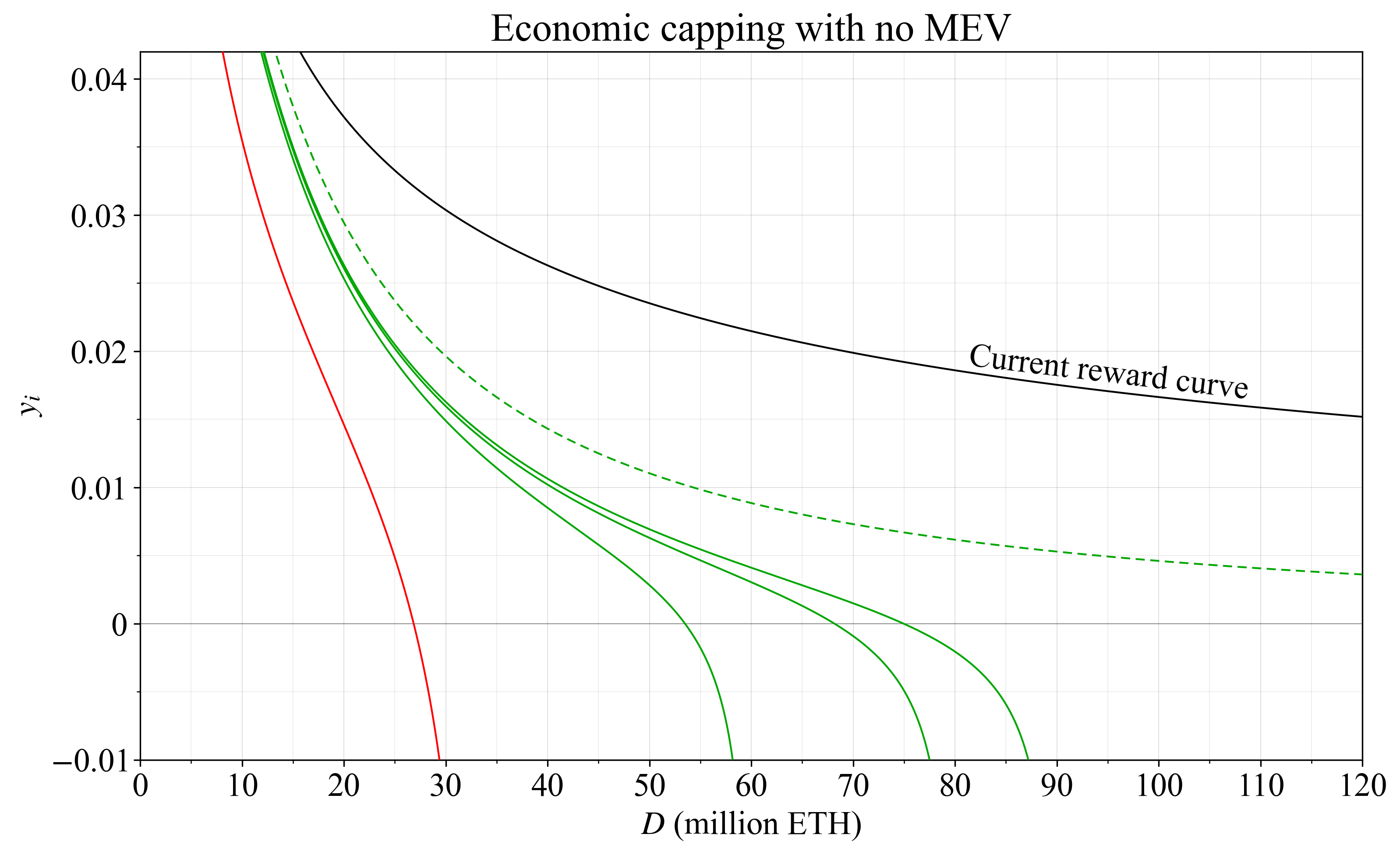
Figure 21. Switching on an economic cap. The reward curve with tempered issuance illustrated by a dashed green line is updated by adding a cap term limiting the quantity of stake to 60M ETH, 80M ETH and 90M ETH respectively (full green lines). Vitalik’s original reward curve for economic capping is shown in red.

5. Time–quantity policy

Adding the dimension of time to the dimension of quantity is also worthy of consideration as an endgame, as described in the last paragraph of Section 6.3 of a previous write-up. Under a time–quantity policy, the reward curve facing the user on shorter time scales can have a moderate predefined shape, but the whole curve is allowed to gradually adapt to changes in the supply curve, implied by the equilibrium. The mechanism is enforced by letting one or two of the variables defining the curve drift as a response to the deposit ratio deviating from some target. This drift can trivially be instituted as a small tick change each epoch, with a size that may or may not depend on the scale of the deviation.

One key realization is that the reward curve variables should change slowly, with larger effects taking place at a time scale of years or even decades. There are a few reasons for this, related to issues discussed in a previous answer when targeting a fixed quantity of stake. Discouragement attacks and cartelization attacks may become less attractive if there is no immediate response in terms of an issuance increase. Furthermore, the protocol will produce a more stable yield if the short-run reward curve is flatter. From a communication perspective, the mechanism always provides a clear trajectory, whereas trying to rely only on time makes issuance trajectories harder to interpret. Finally, the mechanism provides a natural way to transition from one issuance policy to another without causing disruptions. One clear downside is added complexity in the design. As will be shown by the end of this subsection, it is also possible to more strictly retain the notion of budgeting by not relying on a fixed target, instead relying on an underlying target reward curve.

Figure 22 shows yearly issuance under a time–quantity policy. For this example, the reward curve with tempered issuance previously presented was used as a potential starting point in dashed green. A target of 30M ETH is marked by a dark grey vertical line, situated in between the blue crosses. If the quantity of stake is higher than the target, a cap similar to those described in the previous subsection slowly comes into play, gradually shifting the reward curve as indicated in light green, pushing down the yield. Over infinite time, with some fixed supply curve, the equilibrium will be situated either on the grey vertical line or the black curves at the edge that describes the maximum and minimum allowed settings for the reward curve. In this example, that corresponds to the current reward curve as a maximum and a cap at 80M ETH as the minimum (2/3 of the stake). It should be noted that a time–quantity policy does not require that the minimum reward curve institutes economic capping. In a way, this strategy is even more suitable in scenarios where there is no definite guarantee of some cap anyway.

Figure 22. Issuance under a time–quantity policy with a cap. The issuance level will react to changes in the deposited stake along the trajectory of the green reward curves. However, over infinite time scales, if the supply curve is held fixed, the reward curve adjusts such that it enforces an equilibrium along the black path.

The same policy is shown in Figure 23 for issuance yield. On an infinite time scale, the user would be facing a reward curve constituting the upper black curve, followed by the grey vertical line, and concluding with the lower black curve. However, at a time scale of months or perhaps a year or two, the user faces a reward curve along one of the green faint lines, which instantly reacts to direct changes in the quantity of stake. Over time scales of several years, the user faces something in between—a smoothed-out version of the current trajectory, drifting towards the black and grey parts of the reward curve.

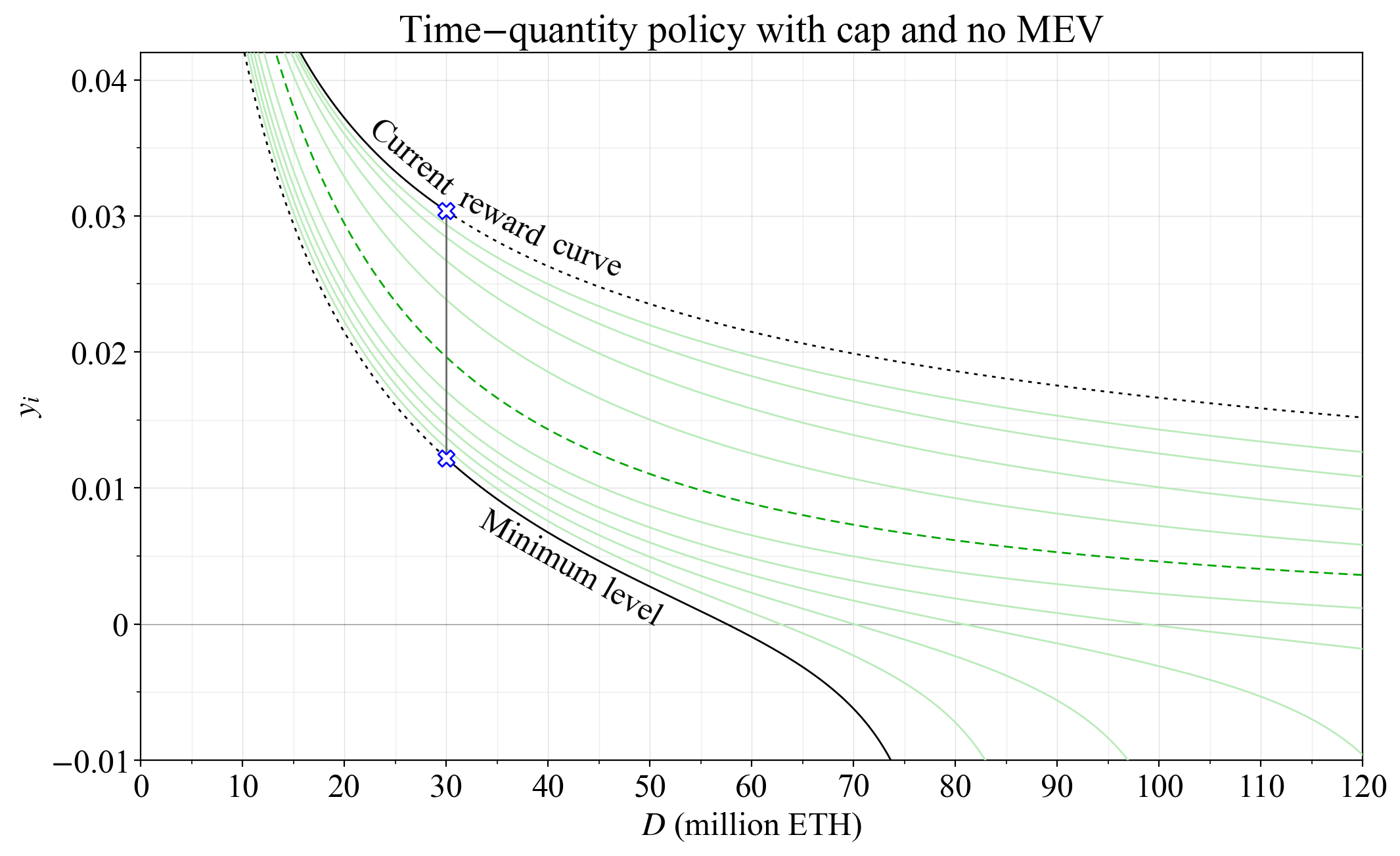
Figure 23. Issuance yield under a time quantity policy with a cap. A further description is provided in the figure text of Figure 22.

One idea behind the time–quantity policy is that the supply curve might slowly fall as the relative costs associated with staking decrease, and that we cannot then enforce some specific quantity of stake over time without having the reward curve close to vertical. As previously discussed, one reason why a vertical reward curve seems undesirable is the high “p_i-elasticity” that it brings.

Even if some specific quantity of stake is optimal, there might also be budgeting considerations in the long run. After all, the notion of not overpaying for security was stipulated as a benefit of using a reward curve in the first place. Figure 24 shows issuance under a smooth time–quantity policy with a cap. It attempts to achieve the best of both worlds: a stricter range in the long run that still has some notion of budgeting incorporated; a flatter reward curve for the short run, moderating fluctuations in yield/issuance, and budgeting based on recent steady states of the supply curve. The black curve is the target reward curve at infinite time scales. In the short run, the protocol will still operate according to a green reward curve, adapting the yield to a change in the quantity of stake.

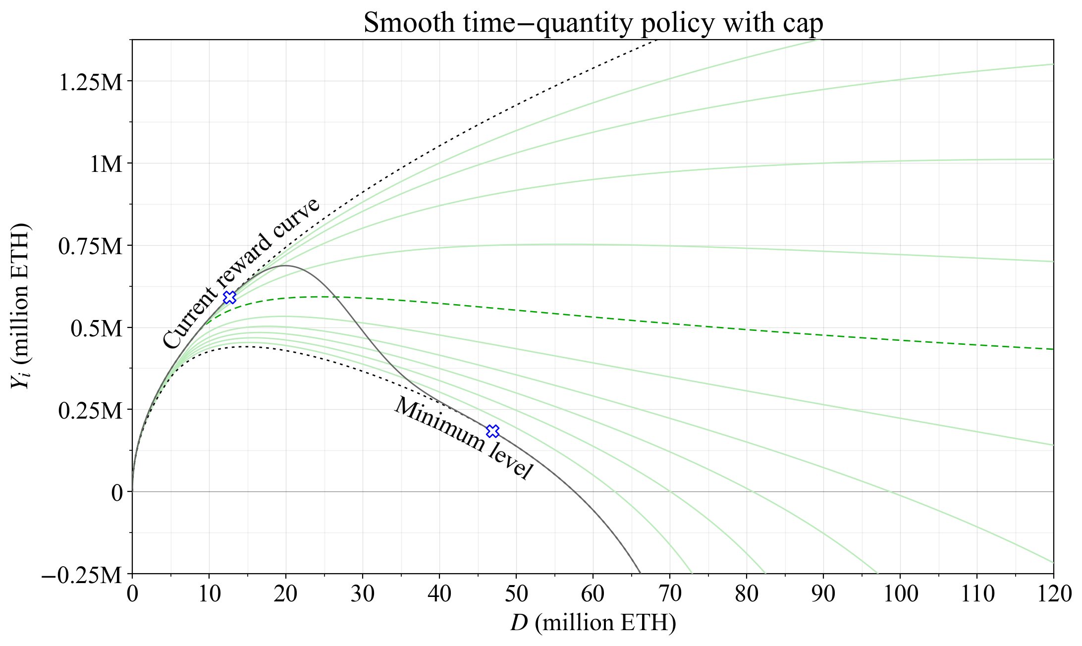
Figure 24. Issuance under a smooth time–quantity policy with a cap. The issuance level will react to changes in the deposited stake along the trajectory of the green reward curves. However, over infinite time scales, if the supply curve is held fixed, the reward curve adjusts such that it enforces an equilibrium along the black path.

The same policy is shown in Figure 25 for issuance yield.

Figure 25. Issuance under a smooth time–quantity policy with a cap. A further description is provided in the figure text of Figure 24.

Time–quantity policies have not yet been researched and debated, and whether or not the added complexity is worth it will be resolved during future discussions.

Why not just prevent new stakers from joining?

Someone in control of a validator then holds a “staking license”, akin to a taxi license or a rental apartment under rent control. This will create side markets, and solo stakers are not necessarily well-suited for navigating those conditions. Such a quasi-permissioned system will generally enable stakers “on the inside” to exercise undue control over the chain and can lead to rent-seeking behavior.

Can stakers profit from a reduced issuance and what is the relevance and impact of the real/proportional yield?

Overview

Stakers hold the underlying ETH, and can profit if an issuance reduction improves Ethereum such that the native asset becomes more valuable. Furthermore, stakers are diluted from newly issued tokens just like everyone else. Therefore, if a high issuance compels many to stake, those that would have staked also at a lower issuance—with fewer stakers competing for the yield—might benefit at a lower issuance. It is by no means certain that the proportion of the ETH that a remaining staker attains will increase from a reduction in issuance (positive y_p as defined below), but any potential loss will be much more modest than what is implied by the change in issuance yield. The condition is illustrated with an isoproportion map in Figure 28.

Welfare gain – stakers as ETH owners

When discussing the effect of issuance policy on stakers, it is first important to recognize that they own the underlying ETH. The native asset of a well-designed decentralized blockchain is more valuable than that of a poorly designed one. In the following subsections, the proportional yield/real yield will be analyzed, accounting for issuance and burn. But it is ultimately Ethereum’s ability to power the world economy that will affect the ETH token holder the most, including the staker. The real “real yield” incorporates the change in value of the underlying ETH—including any staking yield—relative to a relevant consumer price index. It is indeed very useful to have sound native money in an economic system. And the best sound money will not encumber its users to research the reliability of various SSPs, track staking income and see it taxed, or risk being wiped out in a slashing event or other failure.

Proportional yield

Review Figure 26, an updated version of Figure 1. Once again, the effect of a change in issuance under equilibrium is reviewed, with the welfare improvement represented by the dark blue area. The height of the dark grey area represents the loss in yield y for stakers, captured by the red arrow. But when issuance is reduced, everyone is also rewarded with a proportional share of the combined dark blue and dark grey area, in the form of a reduction to the issuance rate i.

The figure illustrates the impact of a change in issuance on ETH holders by taking the dark blue area and the dark grey area and creating a rectangle extending across the full circulating supply (120M ETH). All token holders gain according to the height of this area, shown by an orange arrow. If that height surpasses the height of the dark grey area, the staker will gain a higher proportion of the circulating supply from a reduction in issuance, otherwise it will not.

Figure 26. Implied cost (blue) and surplus (grey) of staking under a hypothetical future supply curve. A change in issuance policy shifts the equilibrium from the black square to the green circle. The cost reduction (dark blue) leads to aggregate welfare improvement as long as the protocol remains secure and decentralized, and the reduction in surplus (dark grey) simply shifts some utility from stakers to everyone. The remaining stakers lose out on yield (red arrow). They however gain from a reduction in the inflation rate (orange arrow), represented by the combined dark blue and grey area extended across the full 120M ETH supply.

The issuance rate is formed as i=y_id, where y_i is the issuance yield and d is the proportion of the circulating supply that is staked. It was indeed the change in both d and y_i that determined the height of the orange arrow in Figure 26 (the change in i). The issuance rate affects the circulating supply inflation rate according to s=i-b. In essence, s captures the percentage change over a year to how many ETH that exist. This means that s rises if the issuance rate is high. Conversely, s falls if a lot of ETH is burned through EIP-1559; this post will use the approximate burn rate b=0.008 since The Merge in the examples. The effect on token holders can be calculated using the equation presented in my thread on minimum viable issuance:

y_p = \frac{1+y}{1+s}-1.

The proportional yield y_p, also referred to as the real yield can be computed for both stakers and non-stakers, in the latter case with y=0. It can be interpreted as the Fisher equation adapted to Ethereum. A simple approximation, applicable at lower yields, is y_p=y-s.

Illustrating the change in welfare and proportional yield

Figure 27 again illustrates what happens under a reduction in issuance to ETH holders, using the same supply and demand curves as in Figure 26. There are three categories: the remaining stakers, the de-stakers between the green circle and black square on the supply curve, and those who were non-stakers already from the beginning. The idea is to compare y_p at the two different equilibria for all token holders, as it changes from y^b_p (black square) to y^a_p (green circle). If y^a_p is higher, the token holder benefits, otherwise it incurs losses. The comparison gives a change in cardinal utility as

u’=\frac{1+y^a_p}{1+y^b_p}-1.

However, one addition is required: use the reservation yield as y for those who stop staking when computing y^a_p. Below that yield, they do not stake anyway, so they suffer no additional loss in utility as the yield decreases further. As shown in the bottom pane, de-stakers will under this definition derive a higher utility at the new equilibrium, with non-stakers clearly better off.

Figure 27. The change in y and s between two hypothetical equilibria is utilized to isolate a change in cardinal utility u' for all token holders. Stakers are subjected to a reduction in yield y, but the reduction in the inflation rate s is similar, so they are left unaffected (y_p stays the same). De-stakers incur no further loss in utility once y falls below their reservation yield. They benefit together with non-stakers from the reduction in s.

The orange arrows in the bottom pane once again illustrate how a reduction in s increases utility for everyone—that’s from removing the dark grey and dark blue areas in the previous figure. The red arrows illustrate how a decrease in yield reduces utility for stakers, corresponding to the height of that dark grey area in Figure 26. For the de-stakers, the red arrows become very short as that dark grey area narrows, even though they forfeited all yield. That’s because their costs went to 0 as well.

The height of u’ thus captures the change in y_p for stakers and non-stakers, and the size of the orange area captures the welfare gain, ultimately deriving from a cost reduction to Ethereum’s users (note that the orange area extends further up to 120M ETH). While stakers may be left unaffected by a reduction in issuance in terms of the proportion of the circulating supply they retain, they can still gain, because the utility of the ETH asset has increased, in accordance with the size of the orange region. The purpose of introducing this figure in my original thread on minimum viable issuance was to encapsulate these insights (welfare gain + proportional yield) in one plot.

The isoproportion map

Clearly the shape of the supply curve will be influential when determining if stakers gain from a reduction in issuance. Stakers benefit from an issuance increase under steep supply curves where no new stakers enter if the yield y goes up. Stakers do not benefit under flat supply curves where a slight bump to the yield makes a ton of new stakers enter, creating circulating supply inflation s in the process. In economics, it is common to use diagrams to illustrate trade-offs by drawing lines along which conditions remain constant, similar to contour lines on a topographical map indicating equal elevation. Figure 28 shows such a map, with “isoproportion lines” indicating where y_p stays the same. Each line is drawn according to the following equation:

y = \frac{y_p-(1+y_p)(v+b)}{1-d-y_pd},\quad \quad y_p<\frac{1-d}{d}.

It is formed by reworking the equation for y_p. The variable v here represents the “MEV rate” constituting MEV as a proportion of the circulating supply. The equation implies the basic condition for profitability that can be imposed on the supply curve under any equilibrium (e.g., via derivation and analysis of elasticities).

Figure 28. An isoproportion map illustrating the conditions under which stakers can attain a higher proportion of the circulating supply from a change in issuance policy. If the slope of the corresponding grey isoproportion line is steeper than the slope of the supply curve under equilibrium, stakers benefit from a reduction in issuance. The red area is at a lower elevation on the map than the orange area even though the staking yield is higher, and thus a worse equilibrium for stakers.

Review the purple dashed isoporoportion line. Stakers get a real staking yield of 1.7% anywhere on this line, although the staking yield and stake participation vary. The red region lies below the line, so ending up there is worse for stakers than ending up in the orange region above the line, even though the staking yield is higher in the entire red region than in the orange region. When nearly everyone stakes, the supply curve must be almost vertical for stakers to benefit from an increase in issuance yield, since the supply inflation rate will increase nearly as much. The orange arrow points towards higher elevation on the isoproportion map, and the ideal equilibrium for stakers lies in the top left corner. But unfortunately for stakers, an equilibrium must lie on the supply curve. Now look at the purple full isoproportion line.

The hypothetical supply curve in blue from the earlier Figures 26-27 intersects both the current reward curves (black) and reward curve with tempered issuance (green) along this line—the equilibria (black square and green circle) are thus at the same “elevation”. This explains why stakers were unaffected in the previous discussion. The highest elevation of the supply curve is marked by a blue star, situated between the two equilibria. At this point, the supply curve is tangent to the corresponding isoproportion line. Plots by Caspar and Ansgar as well as Mike of the green reward curve are useful for showing how its elevation (y_p) varies across stake participation (without incorporating MEV or burn). This is akin to sampling its value from the map across stake participation.

How might the supply curve evolve going forward? Use your intuition to outline its shape and check where your imaginary supply curve reaches the highest elevation on the map (as marked by the star). That’s where the reward curve should intersect the supply curve for stakers to gain the highest proportion of the circulating supply. However, also remember the lessons from the earlier discussion: stakers also gain by holding the native token of a well-designed cryptocurrency that remains secure and imposes low aggregate costs on its users.

Some users think that more yield is more fun and like to collect yield on their ETH. Why not lean into this?

This answer will extend the previous answers (1, 2), and the reader is encouraged to first review them to understand how excessive issuance as well as dilution affects token holders.

The notion of bounded rationality helps to explain why some users may prefer a scenario with lower y_p, where the yield is raised but the supply inflation rate (which users have a harder time to track) rises even more. Behavioral economics can be helpful in this way for explaining why some economic agents act irrationally, perhaps for lack of education or time to deliberate on a topic. But Ethereum should not harness people’s bounded understanding of yield, and keep it high to trick users into thinking that they gain something, when they do in fact not. It is instead important to educate people on these matters so that user utility is not degraded for some hypothetical short-term gain, which is unlikely to materialize. More yield is not more fun. An optimally designed Ethereum is more fun.

Keccak255 · July 6, 2024, 7:22am

Great post!

Considering the current form of the demand and supply curves, where c, c1, c2, and k are constants and D, d, and V are variables that cannot be directly controlled by the Ethereum protocol (though they can be influenced indirectly through new EIPs and other changes), it can be said that from the protocol’s perspective, the supply curve cannot be manipulated, and the demand curve can only be altered by adjusting F.

Overall, can MVI be seen as an “optimization way of d through the manipulation of F”?
And is it correct that the discussion of endgame for issuance levels such as tempered issuance, cut issuance, attempts to optimize d by changing the form of the equation?

aelowsson · July 18, 2024, 11:08pm

Thanks!

Yes. The exact shape of the supply curve is and will remain unknown. New EIPs can also lead the supply curve to shift (for example, if these EIPs make staking easier or harder, riskier or less risky, etc.), but this is not the focus when discussing issuance policy. We primarily have control of the demand curve, specifically the reward curve if we do not institute MEV burn, and more specifically F if no other adjustments to the reward curve are made. However, note that the current direction is to alter the reward curve more substantially, adding other terms to the equation, such as division by the term (1+D/k).

Yes, exactly. As argued in the answer on the endgame, we are seeking to define an optimal path through a set of hypothetical supply curves. Each hypothetical supply curve (both low and high) has one optimal equilibrium, and the reward curve should intersect each hypothetical supply curve close to this point (weighted based on probability). The reward curve should thus optimize all known trade-offs associated with high/low yield and stake participation (long-run and short-run economic security, low costs, a viable composition of the staking set, reward variability, trustless money, low dilution, etc.).