Reward curve with tempered issuance: EIP research post

[aelowsson]

Reward curve with tempered issuance: EIP research post

By Anders Elowsson

My aim with this post is to present the rationale for a reward curve with tempered issuance. It is a longer format of a forthcoming EIP, offering a more detailed account of the benefits and the trade-offs that must be balanced, as well as a comparison with alternative options. I will try to answer any questions you may have in the comments!

1. Overview

Validators began receiving execution layer rewards with The Merge, and liquidity improved when withdrawals were enabled with Shapella. Both upgrades have served to increase the equilibrium quantity of stake. There is a broad consensus that the current deposit size keeps Ethereum sufficiently secure (e.g., 1, 2, 3). Yet issuance will rise substantially as more stake is deposited under the current reward curve. Excessive incentives for staking, beyond what is necessary for security, can unfortunately over time turn into perverse subsidies, with many downsides. This post will explore the benefits of moderating issuance and available options. It concludes that Ethereum should adopt the candidate reward curve, designed to effectively moderate quantity staked while still maintaining reliable consensus incentives, economic security, resistance to discouragement attacks and cartelization attacks, a favorable composition of the staking set, and viable conditions for solo staking. The candidate reward curve divides the equation of the current reward curve by 1+D/k. The single adjusted variable k then comes to define the quantity staked at the peak issuance point, which also corresponds to the point where issuance is halved relative to the current reward curve. A setting of k=2^{26} (67.1M ETH) is suggested as feasible for the near term, with a subsequent potential final adjustment to k=2^{25} (33.6M ETH).

Section 2 – Rationale

The equilibrium yield offered to stakers corresponds to the cost that the marginal staker assigns to staking, i.e., their indifference point between staking and not staking. Section 2.1 shows that if Ethereum offers a higher yield than necessary for maintaining security, it compels its users to incur higher costs, degrading user utility in aggregate. This explains why all ETH holders can benefit from an issuance reduction, something which is also illustrated in Figure 2. The macro perspective is reviewed in Section 2.2. As the quantity of stake grows, one or a few liquid staking tokens (LSTs) may come to supplant ETH as money in Ethereum. Positive network externalities could then lead to both lower user utility and protocol decentralization. Their derivative nature can also erode the social layer’s capacity for upholding Ethereum’s intended consensus process. Section 2.3 suggests that Ethereum should adopt a graduated approach to the proposed changes. Taking a first smaller step will improve Ethereum without being too disruptive, smooth out disequilibria, and allow for an intermediate evaluation of effects on stake composition and quantity.

Section 3 – Proposed reward curve and alternative paradigms

Section 3 presents the proposed reward curve and alternative paradigms. The proposed reward curve is labeled as Option A, with an issuance level that slowly falls as the quantity staked increases beyond desirable levels. Option B sees the issuance level will instead approach an asymptotic maximum. Option C is the current reward curve, with a rising issuance across the full staking range. The options are compared in Section 3.4, showing how the reward curves diverge as the quantity staked increases.

Section 4 – Trade-offs and priors

Section 4.1 explores yield variability for non-pooled stakers and Section 4.2 then reviews how the equilibrium staking yield may affect the proportion of solo stakers. The biggest risk is that disadvantageous economies of scale make solo staking less viable. However, at a higher quantity staked, dominant staking service providers (SSPs) can offer lower fees, better LST money, and lower risk due to emerging moral hazard. The proposed reward curve offers a positive yield across the full range—low enough to make a high quantity stake unlikely, yet sufficiently high as to never force out solo stakers on efficient setups under more improbable scenarios. It is noted that priors regarding both the supply curve and the level of the maximum extractable value (MEV) are relevant to the design. A scenario with a lower supply curve under the current level of MEV is analyzed in Section 4.2.3, aiding the understanding of how the proposed reward curve helps the consensus mechanism absorb delegating stakers with low reservation yields to ensure that solo stakers always are provided with some yield. The broader composition of the staking set is explored in Section 4.3, emphasizing that competition for delegated stake will take place across diverse market segments. Seeing that the cost of running a staking node will not be made prohibitively high relative to the yield, the proposed change will allow variety in preferences and circumstances between delegators to play a more central role in shaping the composition of the staking set. Section 4.4 finally plots the “isoproportion map”, presenting the conditions under which a change to issuance policy is profitable to stakers.

Section 5 – Security considerations

The effects of issuance policy on economic security are discussed both for the short run and long run in Section 5.1. An important reason for providing a positive yield across the full range in the near term is the to preserve consensus incentives without making more extensive adjustments to the protocol, as discussed in Section 5.2. Sections 5.3-4 take a closer look at discouragement attacks and cartelization attacks. These attacks will become more favorable under stricter reward curves where issuance decreases substantially (particularly under a design with negative issuance levels), and are therefore important to keep in mind. The candidate reward curve does not materially exacerbate the risks of these attacks.

Section 6 – Conclusions and discussion

Section 6.1 summarizes the advantages and disadvantages of different issuance levels, and Section 6.2 then presents the author’s conclusion that the proposed candidate reward curve (Option A) is the best alternative for Ethereum at this time. Option C can function as a provisional backup plan. The post concludes by exploring the unknown endgame, broadening the utility measure for token holders to incorporate the development of the entire ecosystem, and cautioning against exploiting users’ bounded rationality concerning yield.

2. Rationale

2.1 User utility

Define the “reservation yield” as the lowest staking yield y at which an individual is willing to stake. Ethereum’s supply curve then emerges from prospective ETH holders’ reservation yields. Figure 1 shows a hypothetical supply curve in blue that will be used in a few examples of this post. Total yearly rewards are Y=yD, where D is the quantity staked (“deposit size”). A holder’s reservation yield can be characterized as the “indifference point” where they derive as much utility from staking as from not staking. The area below the supply curve thus represents the implied aggregate cost to stakers Y_c and the area above represents their surplus Y_s, which combines into total rewards Y_c+Y_s=Y. Relevant costs (broadly defined) include hardware and other resources, upkeep, the acquisition of technical knowledge, illiquidity, trust in third parties and other factors increasing the risk premium, various opportunity costs, taxes, etc. A high yield compels users to incur higher costs than necessary for maintaining security, diminishing user utility in aggregate. Slashing risks or any bugs that would effectively burn the stake are from an “accounting perspective” less attributable as a pure cost at the aggregate protocol level, and taxes will by their nature actually increase costs for a user when its surplus rises. But the general principle of capturing costs below the supply curve as the issuance that does not generate any surplus to stakers is very useful for understanding staking economics and welfare.

A change to Ethereum’s issuance policy from the current reward curve (illustrated in black) to the proposed reward (green) shifts the equilibrium from the black square (1) to the green circle (2). The associated cost reduction Y'_c indicated by the darker blue area benefits all ETH holders, because the ETH was just issued to offset staking costs, without generating any surplus. The shift to the equilibrium also transfers a surplus Y'_s from stakers to all ETH holders (stakers included). The cost reduction is determined by the definite integral of the equation for the inverse supply curve f(x), bounded by the two equilibrium quantities of the comparative static: Y'_c = \int_{D_2}^{D_1} f(x)dx\approx 446k ETH. The surplus shift is instead quantified as Y'_s = D_1y_1-D_2y_2-Y'_c \approx 252k ETH. Thus, almost 2/3 of the issuance reduction directly contributes to welfare improvement, with 1/3 reallocating utility from stakers to all ETH holders. The outcome for a supply curve with a similar shape will be a similar definite integral and cost/surplus respectively. If the supply curve is flatter around the comparative static, Y'_c becomes relatively larger and Y'_s relatively smaller, and vice versa.

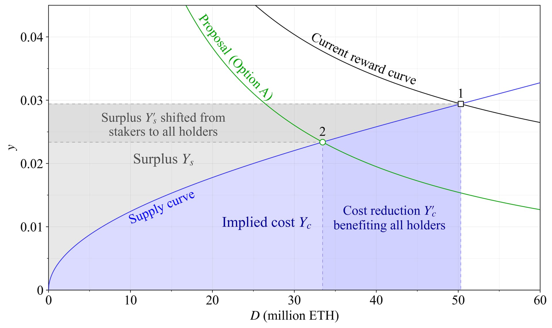
Figure 1. Implied cost Y_c and surplus Y_s of staking with a hypothetical supply curve. A change in issuance policy shifts the equilibrium from the black square to the green circle. The cost savings Y'_c leads to aggregate welfare improvement as long as the protocol remains secure and decentralized, and the reduction in surplus Y'_s simply shifts some utility from stakers to everyone.

Too often, all staking yield is considered as a surplus Y_s, with the implication that issuance policy is a zero-sum game. But due to the costs that must be borne by stakers, issuance policy is emphatically not zero sum. It is fundamental to understand that by having a higher yield, Ethereum steers its users to take on higher costs in aggregate. This is the reason why everyone can gain when keeping issuance at the minimum viable level, as long as they own the underlying ETH.

To illustrate this, the attainable change to someone’s proportion of all ETH can be calculated as

y_p=\frac{1+y}{1+s}-1.

It can be interpreted as the Fisher equation adapted to Ethereum. The “proportional yield” y_p can be computed for both stakers and non-stakers, in the latter case with y=0. The circulating supply inflation rate s=i-b derives from the issuance rate i=Y_i/S and the burn rate b=B/S=0.008, where Y_i is yearly issuance, S is the circulating supply and B is yearly burn (using the average since The Merge). Further complexities regarding the interpretation of rates in light of compounding effects under a drift of the circulating supply are set aside. Figure 2 illustrates the hypothetical effect of an issuance reduction on user utility, utilizing a comparison of y_p at two different equilibria. It is shown here under the proposed reward curve (Option A) and was in previous work presented when halving issuance with the current reward curve (Option C), under a slightly different supply curve. Both y (red arrow) and s (orange arrow) are reduced approximately the same, so stakers are left virtually unaffected. Define the change in cardinal utility for a comparative static where y_p changes from y^b_p to y^a_p as

u'=\frac{1+y^a_p}{1+y^b_p}-1,

but use the reservation yield as y for those who stop staking when computing y^a_p. Below that yield, they do not stake anyway, so they suffer no additional loss in utility as the yield decreases further. As shown in the bottom pane, de-stakers will under this definition derive a higher utility at the new equilibrium, with non-stakers clearly better off. The reason why welfare can improve in this manner is that the staking costs Y'_c of the blue area from Figure 1 are eliminated. Of course, from a protocol perspective, the question of whether solo stakers continue staking or not is also important. This is a separate topic further explored in Section 4.2. The analysis simply concludes that with the hypothetical supply curve, stakers will be left either unaffected (remaining as stakers if they have low reservation yields) or left even better off—as de-stakers. The effect of issuance policy on stakers under any supply curve is illustrated with an isoproportion map in Section 4.4.

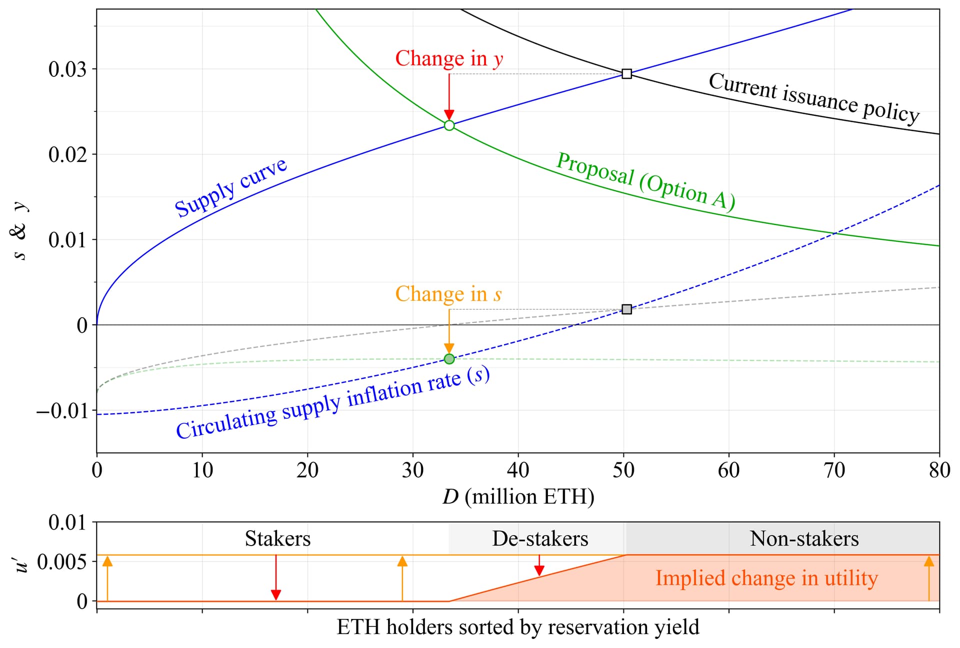
Figure 2. The change in y and s between two hypothetical equilibria is utilized to isolate a change in cardinal utility u' for all token holders. Stakers are subjected to a reduction in yield y, but the reduction in the inflation rate s is similar, so they are left unaffected (y_p stays the same). De-stakers incur no further loss in utility once y falls below their reservation yield. They benefit together with non-stakers from the reduction in s.

Schwarz-Shilling and Dietrich refer to y_p as the “real total staking yield” (they do not specify an equation in their post, but may imply that they use y_p=y-s; with b=0 for visual clarity). Their plots across reward curves, including plots of Option A, are very useful for conceptualizing the measure itself.

2.2 Macro perspective

The reward curve influences the proportion of all circulating ETH that is staked, and it is therefore important to examine the macro perspective of Ethereum’s issuance policy. This can be regarded as one component of a true cost accounting, extending Section 2.1 to incorporate externalities.

An LST exceeding critical thresholds regarding the proportion of stake under its control can gain outsized profits. This stratum for cartelization of block space can ultimately compromise the consensus mechanism. Risks to Ethereum are further exacerbated if an expansive issuance policy (which the current reward curve arguably represents) enables an LST to attain control over a significant proportion of the total ETH—propelled by network externalities of, e.g., the money function. The compromised institution(s) then sits one layer above the consensus mechanism, namely the social layer. It became apparent with The DAO that if the proportion of the total circulating supply affected by an outcome grows sufficiently large, then the “social layer” may waver on its commitment to the underlying intended consensus process. If the community can no longer effectively intervene in the event of for example a 51 % liveness attack, then risk mitigation in the form of the warning system discussed by Buterin may not be effective. The proof-of-stake consensus mechanism has in this case through derivatives grown so interconnected with Ethereum’s users that it has overloaded its ultimate arbitrator, the social consensus mechanism. It is a special and in a way inverted case of issues Buterin previously warned about.

If the issuance policy leads to a high proportion of all ETH being staked, one or a few LSTs may overtake as money in the Ethereum ecosystem, embedding themselves across every layer and application. As has been noted, this is a deliberate objective of some SSPs. By moderating the issuance, each LST will have tougher competition with non-staked ETH, ensuring a trustless asset within the ecosystem. The social layer will not become co-dependent on an outside organization and its issued derivative of ETH. The principal–agent problem (PAP) of delegating stake to a dominant LST can then be priced more accurately because moral hazard will be less likely to develop. No LST will grow “too big to fail” in the eyes of the Ethereum social layer. This pricing will reflect the fact that the agent acting on behalf of the delegator (or any party able to inject themselves into that relationship) gains greater opportunities to degrade consensus for its own profit the larger proportion of the stake it controls. The delegating staker must then continuously assess its security guarantees (e.g., the staking agent’s or injecting parties’ own value at risk), knowing that it may lose everything if the worst-case scenario ever comes to pass.

One cost explored in Section 2.1 can also affect Ethereum at a macro level. In the case where everyone must stake to not see their savings eroded, differences in tax policies across jurisdictions can hamper geographical decentralization.

2.3 Graduated approach

There are a few arguments for a graduated approach, taking a smaller step in the right direction in one hard fork—evaluating the outcome—and if appropriate taking the final step:

• Compromising economic agents’ ability to plan ahead is welfare degrading. While there have been several proposals seeking to temper issuance dating back to at least 2021 (1, 2, 3), individual solo stakers cannot be expected to follow the research debate all too closely. They may first pay attention once a decision has been taken or seriously contemplated. There is also a difference between signaled intentions to moderate issuance and a real decision having been made. A graduated approach is particularly appealing when a change to the issuance policy is implemented relatively shortly after a decision has been made. At the same time, the quantity of stake has at this point already arguably exceeded levels providing sufficient security. Further growth must be considered welfare degrading as well. A graduated approach can in this context:
  • Give solo stakers, and also SSPs, a longer and more gradual adaptation phase.
  • Do something to temper the incentives to stake in the near term, while not being too disruptive.
  • Convey the possibility of additional adjustments to users who may not follow ongoing discussions that closely.
• Ignoring frictions in the decision to stake, a reduction in issuance will precipitate a temporary phase with below-equilibrium yields, until some stakers leave and a new equilibrium is established. A graduated reduction mitigates this problem. An even more gradual reduction, for instance, encoding a small adjustment to issuance every epoch, would bring more implementation overhead.
• It is not possible at this time to ascertain that the full issuance reduction will be necessary to temper the growth in the quantity of stake—it is only a reasonable estimate hinging on assumptions of frictions in the decision to stake or a falling supply curve. Therefore, it seems sensible to move gradually, at least as an acknowledgment of these uncertainties. This reasoning accounts for MEV burn on the horizon, which will also affect the staking yield if implemented.
• There are a few properties of issuance level of particular interest going forward, such as the proportion of solo stakers retained. A graduated approach makes it possible to evaluate intermediate outcomes before implementing the full envisioned issuance reduction. Even if researchers are confident that the full reduction keeps relevant properties in balance, a graduated approach—with an intermediate evaluation before proceeding further—will make the change more palatable to those who may object.

The next section will present reward curves that incorporate a potential intermediate step as part of a graduated approach.

3. Proposed reward curve and alternative paradigms

There are three fundamental paradigms that the reward curve can be designed according to under current circumstances (e.g., absence of MEV burn, no staking fee, and a desire to keep yield variability manageable; see also Section 4.1 and 5.2). These were stipulated in Table 2 in preceding work and are summarized here in Table 1. Option A is the proposed reward curve. It is best at improving user utility and moderating quantity staked, as advocated in Sections 2.1-2.2. Option C provides a higher yield for (solo) staking in the scenario where almost everyone stakes. This may of course also be seen as a drawback, a trade-off further examined in Sections 4.1-4.3. Option B balances between these two approaches. Section 3.4 will plot the reward curves together for further comparison, both for a full reduction and a graduated approach.

	Issuance	Benefit
Option A:	Falls marginally at deposit sizes above sufficient security.	Improves user utility and moderates quantity staked.
Option B:	Asymptotically approaches maximum fixed level.	Balances benefits of Option A and C.
Option C:	Continues increasing indefinitely	Higher yield for solo staking if quantity staked approaches maximum

Table 1. Three main categories for the reward curves, each explored in this section. Option A is the proposed approach, favored by the author.

3.1 Option A – Proposed reward curve

Overview

The proposed reward curve attenuates issuance beyond a quantity of stake sufficient for security. It is designed to give very clear mental models: the value of a single adjusted variable k also defines the quantity of stake at both the peak issuance and the issuance halving point (relative to the current reward curve). The reward curve was presented as the candidate reward curve in a previous post on properties of issuance level. Figure 3 illustrates annualized issuance level across deposit size under perfect validator performance. Issuance of the current reward curve in black varies with deposit size according to the equation Y_i=cF\sqrt{D}, with F set to 64 and the constant c\approx2.6. The grey curve shows halved issuance (F=32). The proposed reward curve in green introduces a division by 1+D/k

Y_i=\frac{cF\sqrt{D}}{1+D/k},

with c and F unchanged. The full reduction is intended to be k=2^{25}, which gives a peak issuance slightly below 0.5M ETH at 2^{25} (33.6M) ETH staked (plus sign), which is also the halving point. The dashed green curve with k=2^{26} (around 67.1M) indicates a potential step in a graduated approach. The fact that the reward curve stipulates a maximum issuance level, which cannot be exceeded, may be beneficial from a communication perspective. In the future, Ethereum’s reward curve shall transition to vary with deposit ratio d=D/S (see Section 6.3), which will then instead translate into a maximum circulating supply inflation rate.

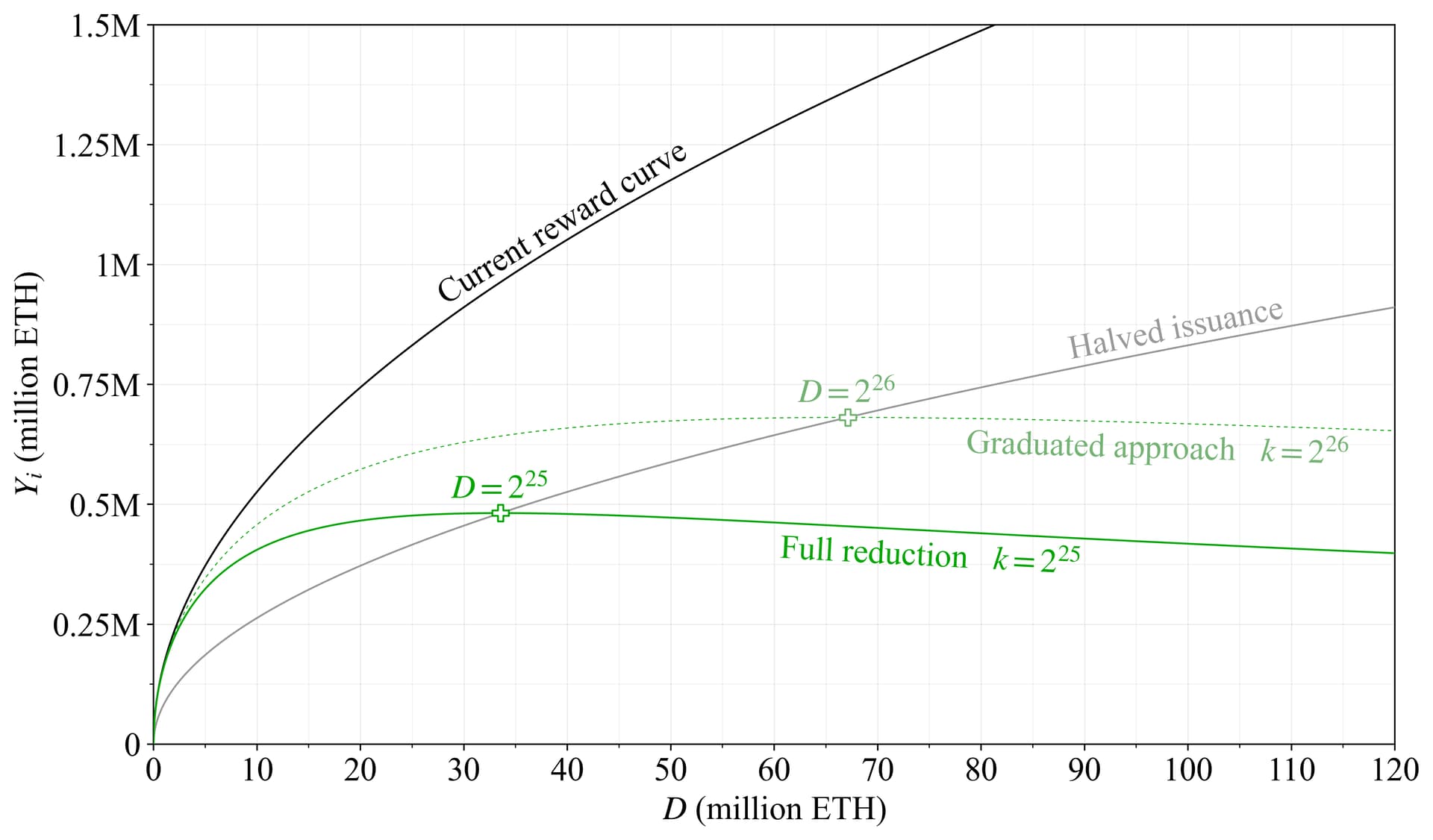
Figure 3. Issuance level for the proposed reward curve—Option A—in green, compared to the current reward curve in black. The dashed green line represents a stepwise reduction in a potential graduated approach. Halved issuance relative to the current reward curve is indicated in grey, with plus signs indicating both halving points and issuance peaks.

Figure 4 illustrates the staking yield in green, assuming a realized extractable value (REV) of V= 300k ETH/year (REV is MEV after builders take their cut and the current prevailing level is slightly above 300k). The equation for staking yield is y=y_i+y_v, with y_i=Y_i/D and y_v=V/D. The equation for issuance yield thus becomes

y_i=\frac{cF}{\sqrt{D}(1+D/k)},

once again multiplying the denominator of the current reward curve (y_i=cF/\sqrt{D}) by 1+D/k. The same hypothetical supply curve as in Section 2.1 is included in Figure 4. It serves to illustrate how the propensity to supply stake may potentially vary across yield and deposit size a few years from now, and what the impact on the staking equilibrium then becomes with an altered reward curve. In this particular example, the equilibrium yield is reduced by 0.6 % (around 1/5), from 2.94 % with the current reward curve (black rectangle) to 2.34 % with the new reward curve (green circle). In the graduated approach, the equilibrium yield is reduced by only 0.43 % (around 1/7).

A reasonable assumption is that the supply curve will gradually shift downwards over time as the staking experience simplifies and DeFi integrations improve. This will in essence depend on how the various costs outlined in Section 2.1 evolve. The faint blue curve could then be the supply curve after another year or two has passed. This would further reduce the yield under both the present and proposed reward curve. The supply curve may also under some circumstances shift upward, for instance, due to a consensus failure prompting stakers to reevaluate risks, or due to increased demand for non-staked ETH, elevating opportunity costs.

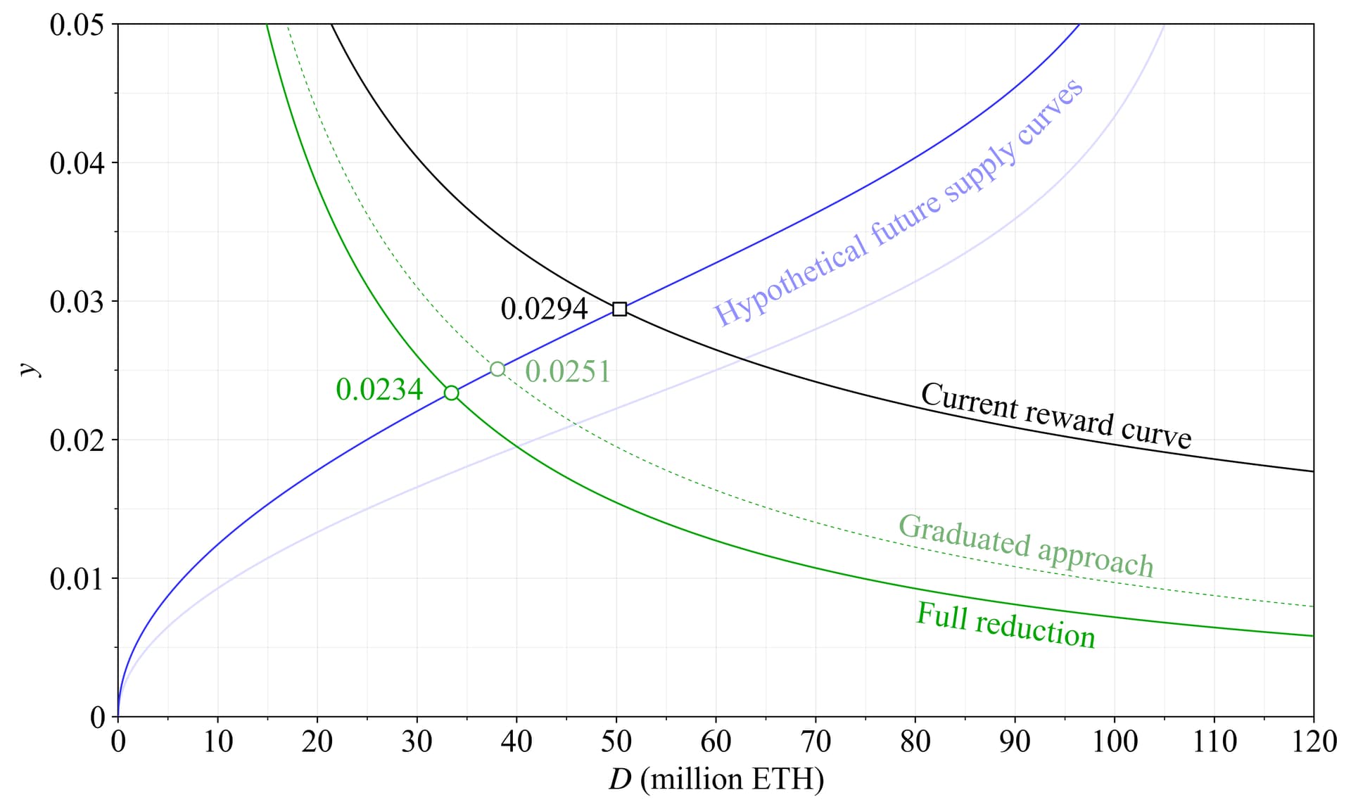
Figure 4. Staking yield (inclusive of REV) for the proposed reward curve—Option A—in green, compared to the current reward curve in black. The graduated approach is depicted in dashed green. Hypothetical changes in equilibrium from the black square to the green circles are indicated as a guideline, but remain speculative due to uncertainty regarding both the supply curve and future levels of REV.

Reward variability

In preparation for the EIP, a simulation of reward variability was performed with current data for REV. Figure 5 shows the simulated cumulative distribution function (CDF) of rewards for solo stakers at various deposit sizes for the proposed reward curve in its full implementation. Figure 6 instead shows the simulated outcome for the graduated approach.

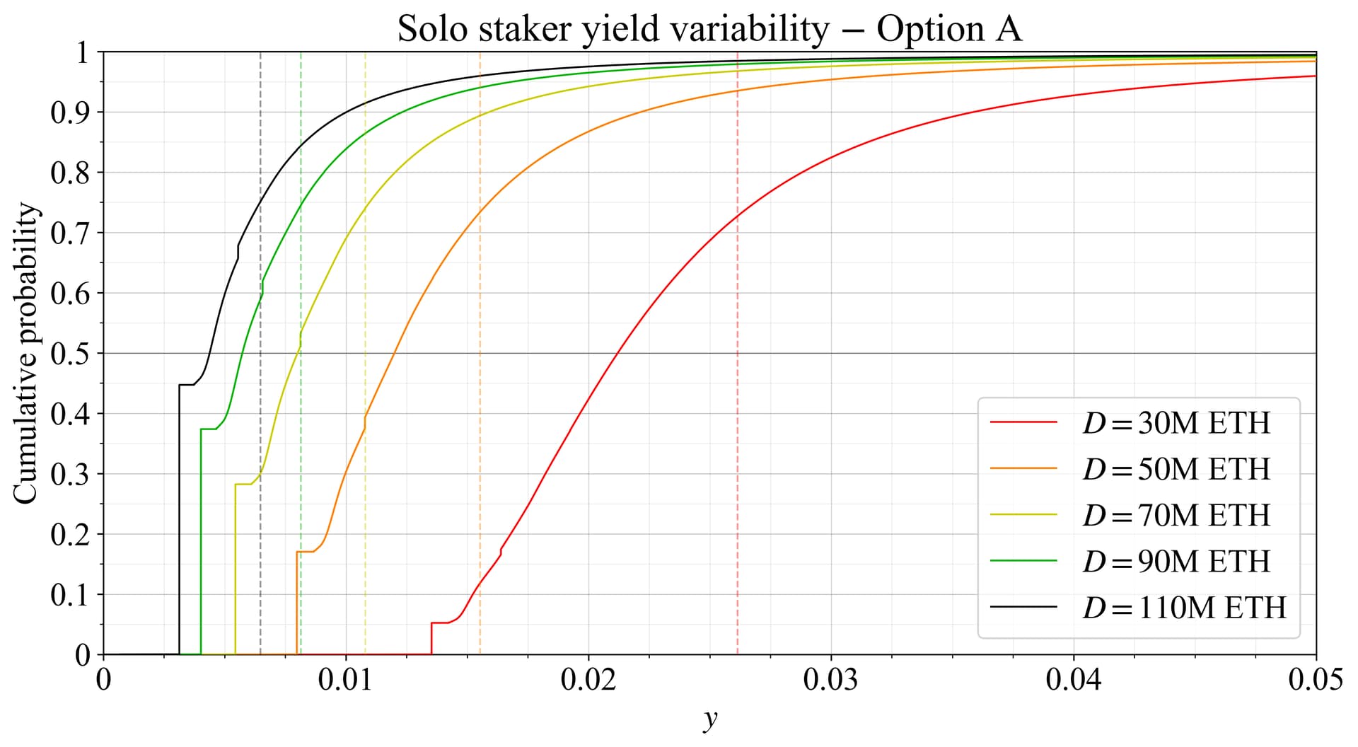
Figure 5. Solo staker yield variability at various quantities staked under the candidate reward curve and present level of REV. Expected staking yields are indicated by dashed vertical lines.

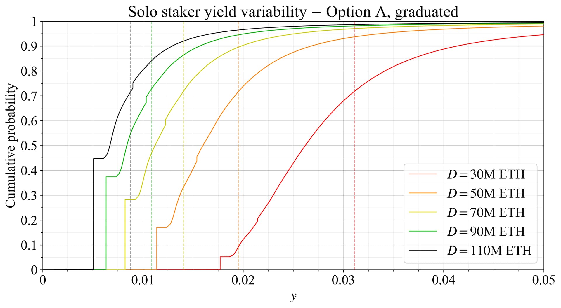
Figure 6. Solo staker yield variability at various quantities staked under a graduated implementation of the candidate reward curve and present level of REV. Expected staking yields are indicated by dashed vertical lines.

3.2 Option B – Asymptotically fixed issuance

Overview

A somewhat more modest option is to instead divide the present reward curve with 1+\sqrt{D}/k, giving an issuance of

Y_i=\frac{cF\sqrt{D}}{1+\sqrt{D}/k}=\frac{cF}{D^{-0.5}+k^{-1}}.

The equation is in essence a log-logistic CDF, and issuance will thus approach an asymptotic maximum of cFk (but it may not come close to that value while Ethereum operates at its current circulating supply). Figure 7 illustrates a potential reward curve for Option B in orange with k=2^{12} and a potential graduated approach with k=2^{13}. As indicated in the figure, the variable F was adjusted to produce a similar issuance as Options A (and Option C) at specific levels, for easier comparison in subsequent sections. Hence, the halving point marked by a plus sign is also around D=2^{25}, and the graduated approach matches the issuance of Option A at the current quantity staked (31M ETH). But F could be re-adjusted to 64, which would increase the probability of an equilibrium at a lower quantity staked.

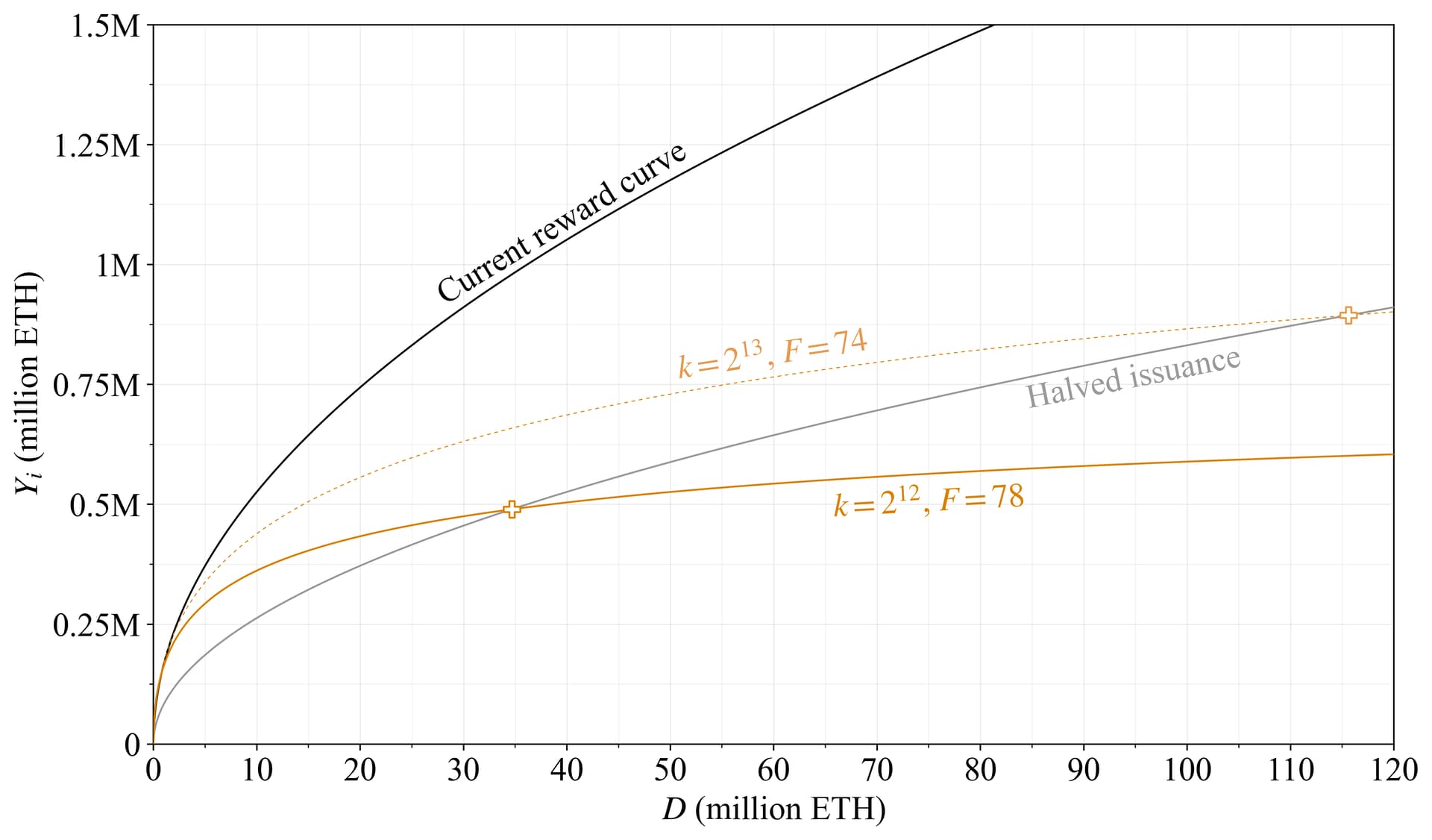
Figure 7. Issuance level for Option B in orange, relative to the current reward curve in black. The dashed orange line outlines a stepwise reduction in a potential graduated approach. Halved issuance relative to the current reward curve is indicated in grey with plus signs.

The equation for issuance yield instead becomes

y_i=\frac{cF}{\sqrt{D}+D/k}.

It is plotted in Figure 10 in Section 3.4 together with the other reward curves.

3.3 Option C – Current reward curve with reduced base reward factor

Overview

The simplest option is to reduce the base reward factor, keeping the current reward curve. The full reduction could then be F=32. It can be noted that this reward curve will reduce the yield relatively more at lower quantities of stake, so F can hardly be reduced below 32 from a security perspective, at least not at this point (see also Section 5.1). A graduated approach should opt for a range between 40-48. In this post, F=44 will be illustrated, since the graduated reward curve will then coincide with all others for easier comparison. Figure 8 plots issuance. Yield is plotted in Figure 10 in Section 3.4 together with the other reward curves.

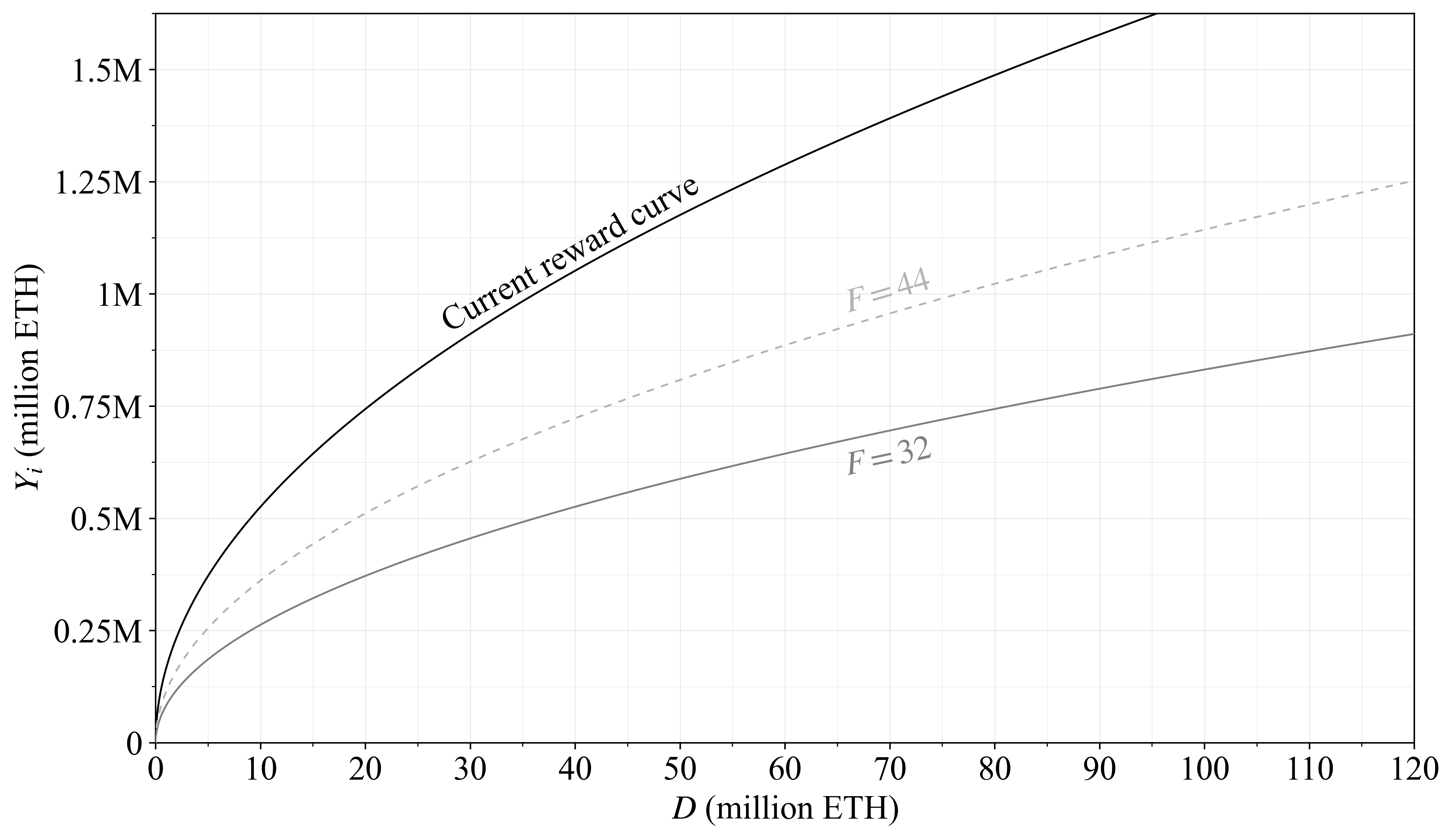
Figure 8. Issuance level for Option C, relying on the current reward curve with a reduced base reward factor. The dashed grey curve indicates a potential setting for the graduated approach. The full possible reduction that retains sufficient economic security is a halving of issuance, indicated by the grey curve.

3.4 Comparison of Options A-C

Figure 9 shows the three outlined options, both for a full reduction and a graduated approach. With the full reduction, all curves coincide around D=2^{25} ETH (circle), above which issuance for Option A declines, B levels off, and C continues increasing. With the graduated approach, all curves (dashed) coincide around the current quantity of stake of D= 31M ETH (star), after which they diverge in a similar pattern. It can be noted that the graduated approach of both Option A and (narrowly) Option B gives a lower issuance if all ETH is staked than the full reduction in Option C.

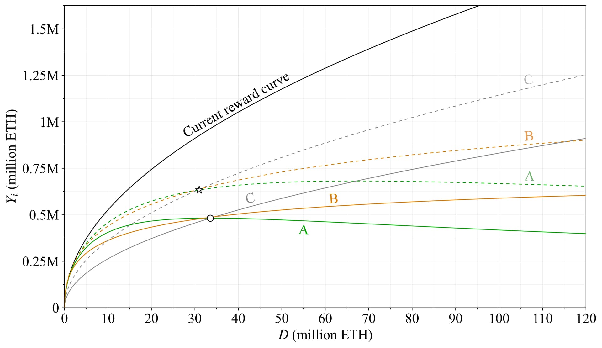
Figure 9. Comparison of issuance levels for Options A-C, with the graduated approach depicted by dashed curves. The three options provide the same issuance at around 2^{25} ETH staked for the full reduction (circle) and at 31M ETH for the graduated step (star), above which issuance for Option A falls, B flatlines, and C continues rising.

Figure 10 shows the staking yield (at the present level of REV) for the same three options. The black double-sided arrow illustrates that the initial reduction in staking yield at the present quantity staked would be under 1 %. The blue double-sided arrows capture the equilibrium shift in yield under the same hypothetical supply curves as previously, demonstrating that the hypothetical reduction in yield would be under 0.5 % for the first graduated step.

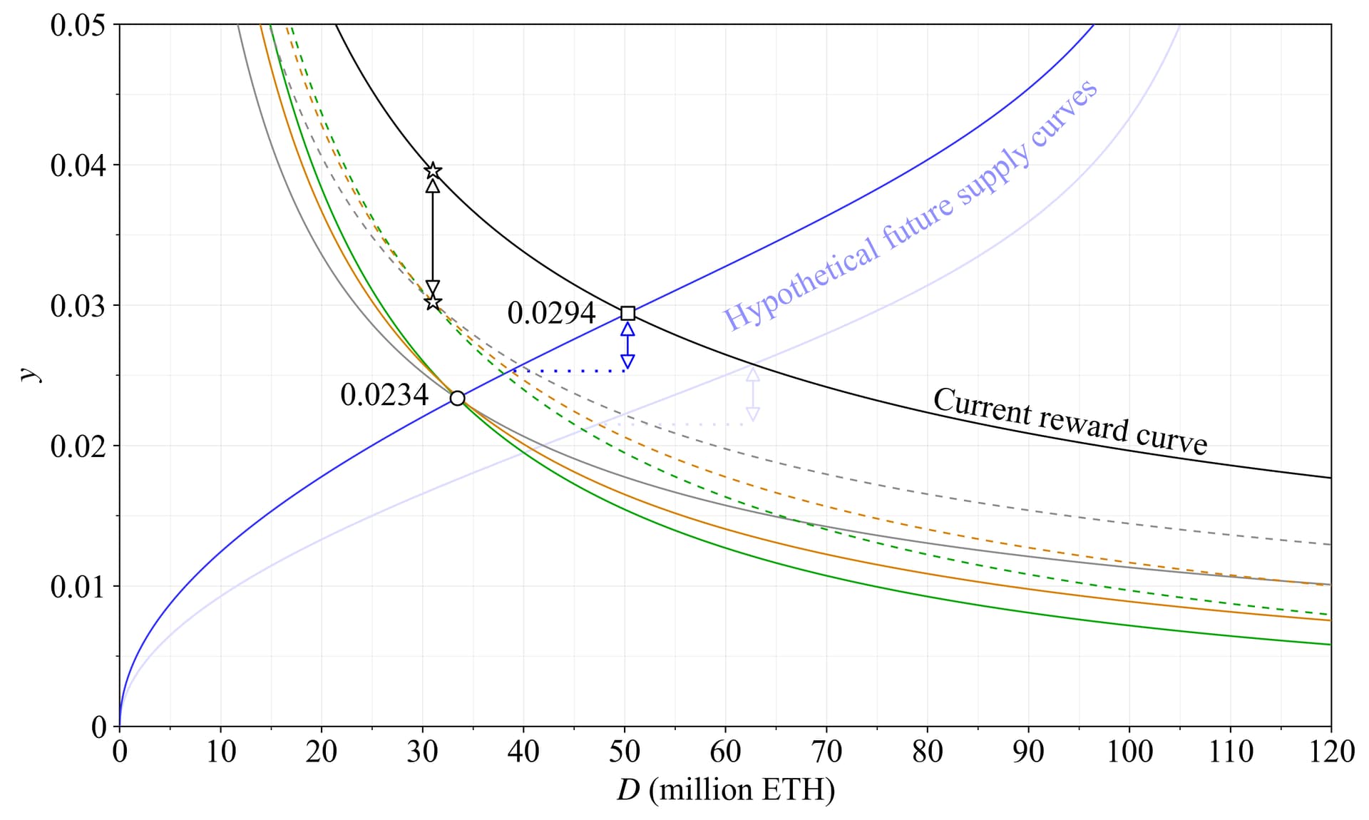
Figure 10. Comparison of staking yield (at the present level of REV) for Options A-C, with the graduated approach illustrated by dashed curves, and the current reward curve in black. A shift in the equilibrium from the black square to the circle is indicated as a guideline, but there is uncertainty regarding both the supply curve and future REV. The initial reduction in the graduated approach is under 1 % (black arrows) and under 0.5 % at hypothetical equilibria (blue arrows).

4. Trade-offs and priors

4.1 Variability for solo stakers

If issuance is moderated, a larger part of rewards will stem from REV, and the relative variability in staking rewards will therefore increase. This affects solo stakers negatively since they cannot effortlessly rely on pooling for smoothing out variability. A simulation of reward variability was performed with current data for REV, resulting in, e.g., the CDFs of Figures 5-6, but also mappings of standard deviations (SDs) of annualized yield across y and D. Recognizing that stakers may be more more sensitive to variance at lower staking yields, the SDs were divided by the square root of the expected yield, referred to as the SSD. This measure attempts to capture degradation from variability for non-pooled stakers. Figure 11 plots the SSD across quantity staked for the different reward curves of this study (lower is better). As evident, the SSD will rise marginally for Option A as the quantity staked increases. This increase is considered acceptable, on the basis that it is reasonable to sacrifice some variability to keep the quantity staked down. When considered in isolation, it is perhaps even desirable to allow the SSD to become a little worse at higher quantities staked than at lower quantities. But having a lower SSD at any D is of course preferable.

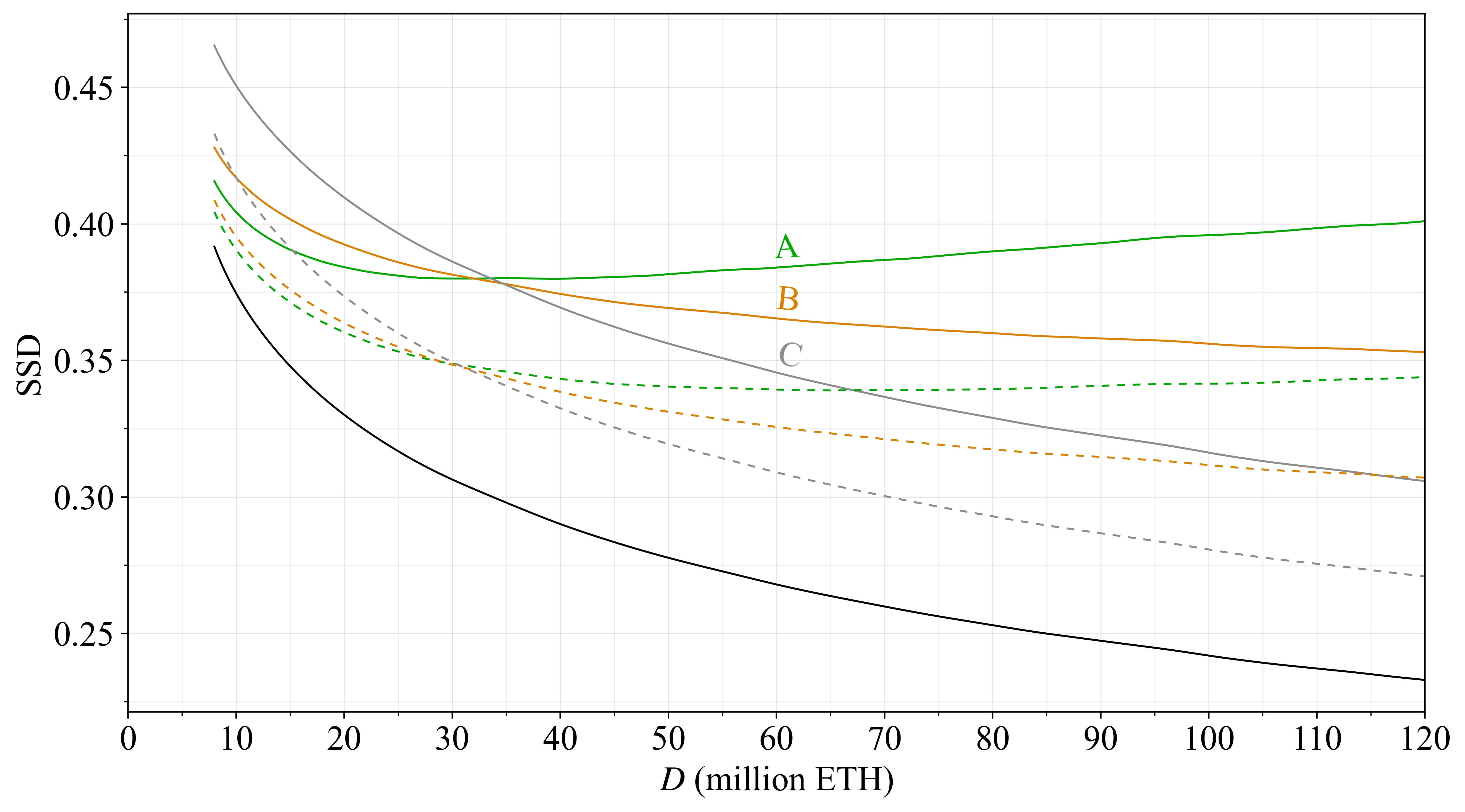
Figure 11. The SSD for the different reward curves (lower is better) across deposit size.

4.2 Equilibrium yield and the proportion of solo stakers

4.2.1 Overview

Ethereum wants to retain solo stakers, certainly at least when measured as a proportion of all stakers. The anticipated outcome of a reduction in issuance level is that less ETH will be staked by both delegating and solo stakers, relative to the outcome when issuance is not reduced (1, 2). Using Figure 10 as an example, it is not clear whether the proportion of solo stakers is lower at a hypothetical equilibrium of around 33M ETH staked and a staking yield of 2.34 % than at around 50M ETH staked and a staking yield of 2.94 %. A concern is if there might be a staking yield below which solo stakers in particular would drop off due to the relatively higher fixed costs associated with solo staking. If solo stakers leave en masse below a yield of 2.5 %, then a staking yield of 2.34 % at 33M ETH staked will give a lower proportion than when the yield is 2.94 % at 50M ETH staked. This is of course something to take seriously. Economies of scale are hard to design away in a decentralized blockchain.

There are however also some arguments as to why a more restrictive reward curve could give a higher or at least similar proportion of solo stakers (see also Section 2.2):

• Dominant SSPs have better economies of scale at higher quantities staked, increasing their cost advantage over solo stakers.
• Likewise, the positive network externality of the money function grows with quantity staked, and with it the competitive advantage of dominant LST-issuing SSPs.
• Furthermore, the PAP associated with an LST may seem less risky if everyone else also uses the LST, with the expectation that the social layer will waver on its commitment to the intended consensus process in the event of a failure.
• Risks could very well price out delegating stakers earlier than solo stakers as the yield falls. If a large enough subset of potential delegators believe that there is a 1 % risk of failure over a year for the LST they wish to hold, then favorable economies of scale or liquidity can be insufficient as a competitive edge. Self-custody is undeniably important to a relevant proportion of ETH token holders; this factor should not be overlooked when evaluating the staking supply side.
• Token holders with enough ETH and the technical ability to solo stake are not necessarily abundant, implying a soft upper bound on the solo staked quantity. It can be argued that if this pool is more or less depleted, then relatively few of the new stakers will be solo stakers as the supply curve falls and D increases under the current policy. Still, concerning this particular argument, it should be remembered that if the yield is reduced substantially to halt the increase in D, there is no guarantee of retaining a larger proportion of solo stakers in the long run. This ultimately depends on the finer-grained distribution of reservation yields among them.

Issuance policy should be focused on long-term objectives and not rely on short-term remedies. This also relates to the presently rather valuable solo staking airdrops, if they can be expected to cease. Yet, Ethereum’s evolving consensus mechanism may look different in ten years, with different requirements for staking anyway—there may even be different classes of validators (1, 2)—so circumstances of the present and in the near-term future cannot be completely ignored. An additional nuance can also be added to the fourth bullet point: some solo stakers stake quite a bit more than 32 ETH, and these may be the most resilient to low yields. Finally note that solo stakers who do not own their hardware may still enjoy some external economies of scale; home stakers on the contrary are directly affected by hardware costs.

At a fundamental level, the conjecture is that the relative distribution of reservation yields may differ between different classes of stakers. This then leads to different proportions of solo stakers under different issuance policies. But whether one policy is better than the other in this respect cannot be ascertained and may also vary over the forthcoming decade. This research topic is certain to receive further attention (1, 2).

4.2.2 Priors regarding the supply curve and REV

Studying the yield offered at 110M ETH staked in the CDF of staking yield for Option A in Figure 5 may raise particular concerns. The expected staking yield there is only 0.65 %. At a token price of around $3000, a 32 ETH stake would then only generate an expected monthly income just above $50. The “guaranteed” attestation yield not deriving from block proposal or sync-committee duties is only half of that. A decline in the ETH token price could further reduce the income from staking. However, it should be noted that a reasonable prior for the supply curve is that the yield must be quite a bit higher than 0.65 % for 110M ETH to get staked. The only time an equilibrium can be expected at 110M ETH staked is then if the REV increases significantly, pushing up the staking yield to required levels. One easily overlooked benefit of a lower issuance yield at high quantities staked is thus that it pre-emptively counters a higher REV (the staking yield will never go below the marginal staker’s reservation yield under equilibrium). Concerns may of course also be raised around the fact that the quantity of stake is allowed to expand to 110M ETH in the first place, given the good arguments against it. Why offer any yield at all? Besides care for solo stakers, important reasons pertaining to consensus incentives at the present are provided in Section 5.2.

4.2.3 Low-yield scenario

While it seems probable that a high quantity staked under the proposed reward curve (Option A) would be associated with an elevated level of REV, thus maintaining a slightly higher staking yield, it can still be valuable to examine the alternative scenario. What if the supply curve indeed falls substantially over the next decade to a very low level? Option A gives a staking yield to 1 % at around 74.6M ETH staked under the current level of REV. Option B gives a staking yield of 1.16 % there, and Option C sets it to 1.37 %. But the equilibrium would of course shift to a higher quantity staked for Option B and C, reducing the yield a bit in the process. A hypothetical outcome for Options A-C in a scenario with an equilibrium yield of 1 % for Option A (green circle) is shown in Figure 12. It is of course challenging to speculate on what the supply curve might look like in this unlikely scenario, but it may still be helpful to plot one possible outcome to aid the understanding (it is formed as in the previous study using k=1 and c_2 = 0.001). Option B then gives a yield of 1.09 % at an equilibrium of around 80M ETH staked (orange circle) and Option C gives 1.24 % at around 87M ETH staked (grey circle). Which outcome is better for Ethereum?

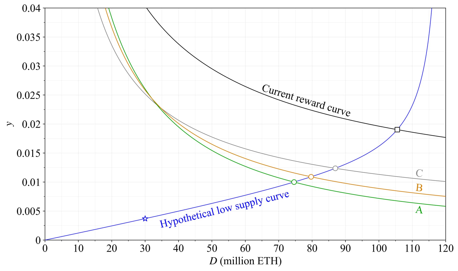
Figure 12. Hypothetical equilibria in a scenario with a low supply curve that intersects 1 % staking yield of Option A under the current level of REV.

If many solo stakers have a reservation yield between 1.24 % and 1 %—in this particular scenario where the majority is staked with reservation yields below 1 %—then they could be disproportionately more likely to drop off. This goes back to the trade-off between the relatively higher fixed costs for solo stakers and the benefits of LSTs at high quantities staked: the notion that dominant SSPs can offer lower fees, better LST money, and lower risk due to emerging moral hazard.

Ethereum can be designed to enforce an equilibrium at any point along the supply curve (but must be attentive to the level of y_i relative to y_v). Would enforcing an equilibrium at the blue star be preferable under this supply curve? It corresponds to 30M ETH staked and a total staking yield of around 0.37 %. At present, y_v is 1 % at 30M ETH staked, so a staking fee would need to be introduced and taken out every epoch. This would require making solo stakers lose money every epoch, on the slim chance that they may be assigned to propose a block. That outcome is rather unappealing. But what about after introducing MEV burn, would it be desirable at that point? There are several arguments in favor of it (e.g., Section 2), but it could also render solo staking rather disadvantageous due to the relatively higher fixed costs. The effect on the composition of the staking set is harder to predict when enforcing a low quantity staked in such a manner at this point (refer also the next subsection). If the equilibrium yield is 2.6 % at 30M ETH staked, as with the candidate reward curve, then the outcome is far less controversial. An upward shift to the equilibrium quantity of stake—from the blue star to the green circle—acts as a “safety valve”, which helps Ethereum neutralize the less desirable properties of a low quantity of stake under a lower supply curve. The consensus mechanism essentially absorbs all delegating stakers with low reservation yields, just to push up the yield enough to allow solo stakers to still operate a 32 ETH validator at a profit. Regardless of whether this is desirable or not, for the sake of users, the upward shift must only take place if strictly required. This is something that the reward curve facilitates.

It can be interesting to note the difference between the proposed Option A and the current reward curve also under this hypothetical supply curve. The staking yield at the black square in Figure 12 is around 2 % and the incentives to stake thus much higher, drawing 105M ETH into staking. The downsides are the same as previously discussed. Everyone is forced to stake to not see their savings eroded. The issuance level at the black square is around 1708k ETH per year, i.e., almost four times higher than under Option A. Therefore, even though the yield increases by almost 1 %, the supply inflation rate increases even more. Thus, remarkably, stakers are still left worse off under the current reward curve than under Option A, and everyone loses in terms of u'. This follows from the fact that the gain in y_i does not materially surpass the loss from the increased issuance rate i=y_id, where d is the deposit ratio d=D/S. Thus, for an increase in issuance to be profitable at high deposit ratios, the supply curve must slope almost vertically upwards, as further explored in Section 4.4 and Figure 14.

In the example in Figure 12 with a low supply curve, changing from Option C (grey circle) to Option A (green circle) reduces issuance by around 330k ETH, from around 775k ETH down to 446k ETH. Around 42 % of that reduction corresponds to decreased implied costs Y'_c. The change in utility for ETH holders is shown in Figure 13. Everyone would be better off at the equilibrium of Option A than Option C (disregarding frictions). However, as previously mentioned, this does not mean that solo stakers will keep staking. They could be even better off de-staking, if their reservation yield sits in between 1 % and 1.24 %. From a macro perspective, the overall protocol (including the ETH token holders) could then be worse off if the proportion of solo stakers falls too much. The macro perspective is further interwoven with user utility in Section 6.4.

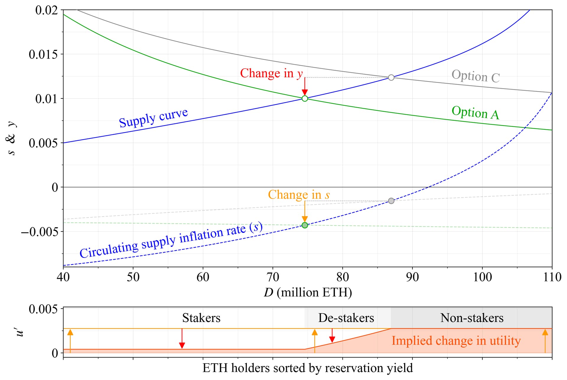
Figure 13. Isolating the change in utility u' when changing from Option C to Option A under a low supply curve. Stakers are subjected to a reduction in yield y, but the reduction in the inflation rate s is larger, so they are left slightly better off. De-stakers incur no further loss in utility once y falls below their reservation yield. They benefit together with non-stakers from the reduction in s.

4.3 Equilibrium yield and the broader composition of the staking set

The relationship between issuance level and diversity in SSPs also entails a trade-off between economies of scale and factors such as the positive network externality of the money function. The fact that a positive yield is offered across the full staking range helps alleviate concerns that a major SSP with a structural advantage such as a centralized exchange (CEX)—perhaps leveraging some hypothetical staked ETF—can push up their proportion of the stake to critical levels. At the same time, the risks of centralization around such entities should not be disproportionately emphasized over other risk scenarios. There are already today SSPs attaining critical proportions of the stake by leveraging network externalities onchain, ostensibly foregoing profits in the pursuit of monopolization. This type of structural advantage grows with higher issuance, and stifling that before native ETH possibly is in the minority relative to one LST must be considered as a net positive to the community. When weighing these trade-offs, an issuance level that invariably forces any outcome—whether a very low or very high quantity staked—does not seem desirable. Just as when discussing solo staking, if the supply curve indeed is very low, then it seems acceptable to let the deposit size grow a bit above a level sufficient for security so that some staking yield still exists. If the supply curve turns out to be rather high, then a low deposit size is perfectly fine. No SSP can reasonably outcompete all others if there is an equilibrium at a 2.6 % staking yield and 30M ETH staked (as with Option A).

Each SSP, reaching for a specific market segment, incurs unique costs besides the cost of running staking nodes, with a wide variety ranging from compliance to software. Indeed, CEXes have somewhat of a local monopoly on their customers-as-delegators, and the opportunity cost of keeping fees competitive with any onchain option is presumably so high that it does not represent the profit-maximizing strategy. What is clear is that competition for delegated stake will unfold across diverse market segments, and perfect competition is not a reasonable assumption. Seeing that the cost of operating a node will not be made prohibitively high relative to the yield, the proposed reward curve (or any of the other options) does not explicitly force a low quantity staked, ultimately allowing variety in preferences and circumstances between delegators to take a more central role in shaping the composition of the staking set. There is therefore no compelling argument as to why any one SSP will overtake others under Option A, B, or C. This is especially pertinent when adopting a graduated approach and evaluating the outcome before proceeding further. There is also already the risk of centralization being more likely under the current reward curve, in this case leveraged by some emerging dominant LST as the money of Ethereum.

4.4 The isoproportion map

Figure 14 maps y_p for stakers across y and D under the previously specified burn rate b=0.008 and annual REV V= 300k ETH. The thin black lines can be characterized as “isoproportion” lines across which y_p remains constant (refer to the equation below). The isoproportion map is essential for stakers attempting to understand the effects of issuance policy on their share of the circulating supply. If the slope of the supply curve is steeper than the associated isoproportion line at some specific equilibrium, stakers benefit from an increase in issuance (u'>0); if it is flatter, they are worse off. In microeconomics, a “production possibility curve” can be compared with isoprofit lines to optimize a production set. To the staker, the supply curve becomes a “proportion possibility curve” (the PPC of staking economics), capturing how stakers’ attainable proportion of the circulating supply varies with issuance policy.

Two hypothetical supply curves are shown in blue, the low supply curve from Figure 12 (dashed) and the baseline supply curve from previous figures (full). The purple isoproportion lines intersect the equilibria of the current reward curve (squares). Since the supply curves (the PPCs) have a flatter slope at equilibrium, stakers are worse off from an increase in issuance, and thus benefit from a decrease in issuance in both cases. They are clearly better off (higher y_p) under the low supply curve at the equilibrium for the proposed reward curve (green circle), and left indifferent under the baseline supply curve (as also indicated in Figure 2). The stars mark where the supply curves reach their maximum y_p, tangent to the corresponding isoproportion lines. This is the ideal equilibrium in terms of y_p for stakers. All other token holders would of course still gain from a reduction in issuance, so in terms of u', they would certainly prefer an equilibrium at 20M ETH staked under the low supply curve (triangle), where stakers are just as well off as at the outset at the square.

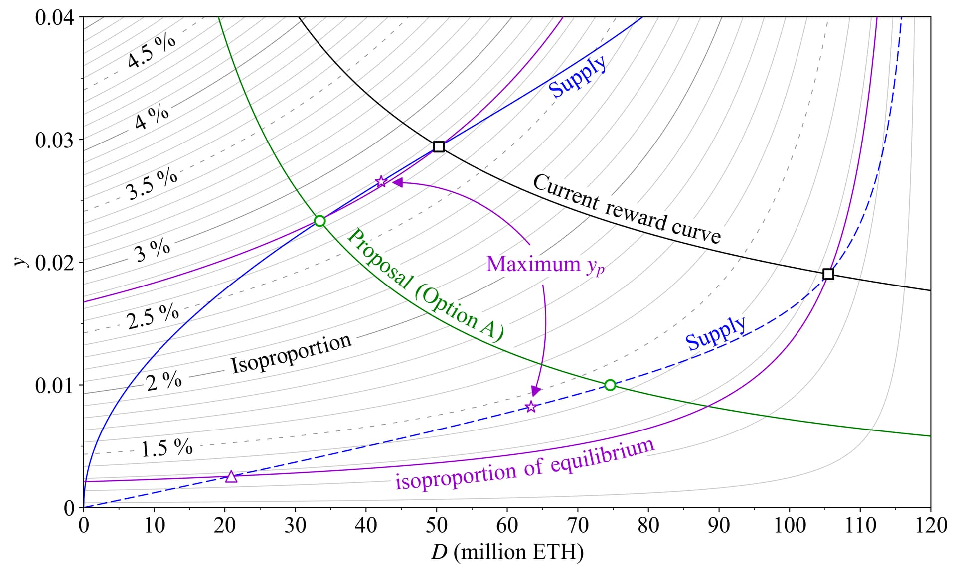
Figure 14. Isoproportion map that illustrates the effects of issuance policy on staker’s proportional yield y_p under equilibrium. A reduction in issuance from the current reward curve (black) is profitable to stakers under both hypothetical supply curves, because the purple isoproportion lines have a steeper slope at equilibrium. The stars indicate the maximum attainable y_p along the supply curves.

Define v as the REV rate v=V/S. The isoproportion line for any specific y_p then follows the equation

y = \frac{y_p-(1+y_p)(v+b)}{1-d-y_pd},\quad \quad y_p<\frac{1-d}{d}.

This equation implies the basic condition for profitability that can be imposed on the supply curve under any equilibrium (e.g., via derivation and analysis of elasticities). If the (inverse) supply curve follows this equation (along any specified y_p), stakers will be indifferent to a change in issuance across the whole deposit ratio range.

5. Security considerations

5.1 Economic security

There are certain critical thresholds to be attentive to when reasoning about the economic security of Ethereum. An attacker holding more than 1/3 of the stake can delay finality, an attacker holding more than 1/2 can control the fork choice, and an attacker holding more than 2/3 of the stake can finalize the chain. Each of these attacks would cause severe disruption, but comes at a great potential cost to an attacker. In the case of a delay to finality, the attacker is subjected to an inactivity leak. The cost of causing loss of finality for some specific amount of time in some specific way scales linearly with the total deposit size, and quadratically with time. An offline validator leaks around half their ETH in a little less than three weeks during an inactivity leak. A complete cost analysis for causing loss of finality (and other attacks) also needs to account for price movements on the ETH that an attacker necessarily must control. An attacker may both lose ETH and see the value of any ETH they still retain diminish—if the attack causes real damage to Ethereum. For attacks made possible by holding more than 1/2 or 2/3 of the stake, it is a natural assumption that the social layer would intervene. The ultimate recourse would then be to burn some or all of the attacker’s stake.

When it comes to attacks from a smaller stake, there are several reorg attacks and minority discouragement attacks (Section 5.3) to take into consideration. Many of these attacks also depend on the proportion of the stake held by an attacker (i.e., holding 25 % of the stake opens up more avenues than holding 0.1 %). From this brief review, it becomes evident that the quantity of stake cannot be allowed to become too small, because the cost of causing severe disruption to Ethereum would then not match the damage done. Table 2 denotes the cost of 1/3, 1/2 and 2/3 of the stake at a token price of $3000 under a deposit size of 14M ETH (the deposit size at The Merge), 24M ETH (20 % of the stake), and 30M ETH (close to the current deposit size).

	1/3	1/2	2/3
14M	$14B	$21B	$28B
24M	$24B	$36B	$48B
30M	$30B	$45B	$60B

Table 2. Value at risk for the critical proportions 1/3, 1/2 and 2/3 of the stake at a token price of $3000 across a few relevant deposit sizes.

While present fiat-denominated costs of potential attacks at various deposit sizes are interesting to review, Ethereum’s economic security will in the long term inherently be linked to the ability of ETH to retain its value. A holistic perspective is therefore important also when considering economic security. This is underscored by reflecting on the early days of Ethereum, when the ETH token was much less valuable. Eight years ago, In May 2016, Buterin deliberated on the value that Ethereum can and cannot secure at a deposit ratio of d=0.3. At the time, the market cap of the ETH token was roughly 500 times lower than today, and the economic security that Ethereum could offer was therefore limited. Increasing the deposit ratio from 0.3 to 0.6 would only increase the value of 1/3 of the stake from $70M to $140M. This highlights that once the deposit ratio has risen above insignificant levels, it will ultimately be Ethereum’s role in the world economy, and the ether’s role in the Ethereum economy, that determines the economic security. Insights from all sections of this post, including the forthcoming Section 6.4, must thus be considered when settling on a suitable deposit ratio. This is a complex task that cannot be objectively formalized. Note in particular that the level of the staking yield—when considered in isolation—will not be a determinant of the value of the ETH token and thus Ethereum’s economic security, as the yield comes from newly minted tokens, directly diluting holders.

There comes a point where the marginal increase in security from adding another validator brings less utility than the utility loss stemming from the numerous downsides of excessive issuance previously outlined. This point hints at a desirable deposit ratio. Justin Drake suggested that d=0.25 (30M ETH) is appropriate in a recent AMA on Reddit. Vitalik Buterin concurred, elaborating on factors influencing the broader composition of the staking set along the lines of Section 4.3, but also added a personal note of finding d=0.125 (15M ETH) fine. As the quantity of stake grows, the prospects for high economic security in the long term gradually begin to diminish. It seems perfectly reasonable to argue that Ethereum would have higher economic security twenty years from now with a reward curve that sees the deposit ratio settle on d=0.25 than at d=0.75—as long as the composition of the staking set remains viable. When the deposit ratio grows beyond certain limits, even short-term security starts to degrade, in line with the reasoning in Section 2.2. The social layer may lose its neutrality and credibility as the ultimate arbitrator against attacks from dominant SSPs. At the other end, it also seems reasonable to ensure that the deposit size does not fall below 14M ETH, which was the prevailing size at The Merge (or more accurately, that the deposit ratio does not fall below d\approx0.12). Such a lower boundary at least ensures that Ethereum never ventures into unknown territory in terms of stake participation (as previously discussed, it is impossible to ensure that the value of the stake is kept at some specific level relative to the value secured).

The discussion of economic security has underscored the complexity involved in determining the correct deposit ratio. As a matter of fact, due to uncertainty regarding several key variables, there is not one specific ratio that always maximizes overall utility. The most suitable deposit ratio will arguably vary with the shape of the supply curve and the cost of providing a certain level of security. If the implied costs associated with staking are higher (as captured in Figure 1), then it seems reasonable to have a slightly lower deposit ratio than if the cost is lower. This is one of the reasons for using a reward curve in the first place—it allows Ethereum to adjust the security level based on the price of that security. Ethereum should thus target a deposit ratio range, which can be rather broad, allowing the supply curve to influence the equilibrium quantity of stake. The proposed reward curve—in the author’s view and under full implementation—balances the many needs of Ethereum, including viable economic security for the short term and possibly the long term (see Section 6.3 for additional nuances).

Table 3 shows the yield that the protocol will provide at the previously discussed deposit sizes, given the current level of REV. In addition, the outcome if the REV was to completely vanish is also provided. Note that if Ethereum ever adopts MEV burn and there is a clear need for it, the associated hard fork can apply dedicated adjustments for re-calibrating issuance. On the other hand, should the supply curve fall over the next few years and there is an agreement within the community, then the introduction of MEV burn can be conceived as the last step in the moderation of the quantity staked.

	A: y_i	y_i+y_v	B: y_i	y_i+y_v	C: y_i	y_i+y_v
14M	3.14 %	5.28 %	2.83 %	4.97 %	2.22 %	4.37 %
24M	1.98 %	3.23 %	1.88 %	3.13 %	1.70 %	2.95 %
30M	1.60 %	2.60 %	1.58 %	2.58 %	1.52 %	2.52 %

Table 3. Staking yield at various relevant deposit sizes under the full reduction in issuance.

The first column indicates that the quantity staked will stay at healthy levels under Option A, even without REV. It seems reasonable to assume that at least 24M ETH would still be staked at a 2 % yield. Certainly, 14M ETH would still be staked if a 3.1 % yield is offered. However, if this were to be a concern for some reason, the option would then be to move back the peak of the reward curve slightly, while raising F. For example, the graduated approach could then have a k between 25M to 2^{25} and the full reduction around 20M; both with a base reward factor in the vicinity of 10^{2}. The lower yield under Option C can be noted, and is one of the reasons why a base reward factor below F=32 is undesirable from a security perspective for this option. Table 4 instead shows the outcome under a graduated approach.

	Ag: y_i	y_i+y_v	Bg: y_i	y_i+y_v	Cg: y_i	y_i+y_v
14M	3.68 %	5.82 %	3.53 %	5.67 %	3.06 %	5.20 %
24M	2.50 %	3.75 %	2.46 %	3.70 %	2.33 %	3.58 %
30M	2.10 %	3.10 %	2.10 %	3.10 %	2.09 %	3.09 %

Table 4. Staking yield at various relevant deposit sizes under a graduated approach.

5.2 Consensus incentives

A reduction in issuance will alter the balance between the various roles that consensus participants are assigned to. In particular, the proposer will attain a larger proportion of all rewards, and this may threaten consensus stability. If the yield provided for attestation duties y_a becomes a small proportion, y_a/y, of the staking yield, stakers can be expected to pursue irregular and adverse activities when profit-maximizing, and the consensus process may break down. They may as an example even stop attesting entirely to avoid the risk of slashing. The proposed reward curve has been designed to give attesters at least half of the rewards at any deposit size under the current level of REV, as illustrated in Figure 15. Should the REV rise substantially, the penalty for a missed target vote (and potentially source vote) can be raised, to give proper incentives for performing attester duties correctly.

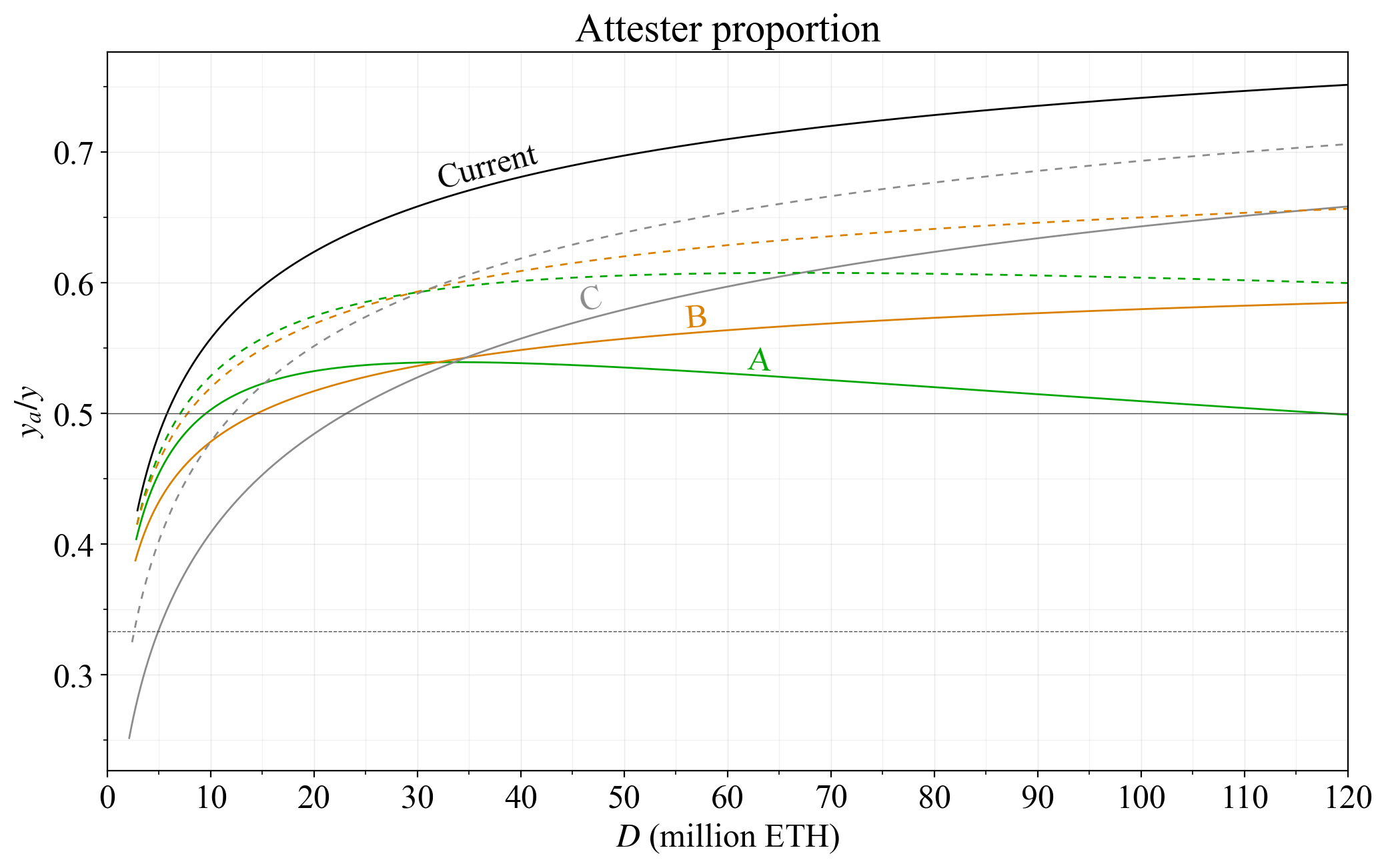
Figure 15. Proportion of the staking yield provided for attestations (y_a/y) under 300k ETH REV/year for the analyzed options (graduated approach in dashed lines).

5.3 Discouragement attacks

A discouragement attack is a malicious action against honest consensus participants of a blockchain, potentially at a cost for the attacker, to profit from the reduced competition for the remaining rewards. The traditional scenario outlined by Buterin involves a majority attack, but there are currently a few possible minority discouragement attacks against Ethereum. These include the censorship of sync-committee attestations, withheld attestations during an inactivity leak, and censorship of the head and potentially source vote (picking up stray votes in subsequent slots). Withheld attestations during an inactivity leak are a special case, because the attack is directly profitable. Since the victim loses out on seven times more ETH than the attacker and also receives a penalty of equal size as its loss, censorship of sync-committee attestations has a griefing factor of G=14.

The “p-elasticity”—capturing the negated inverse point-wise yield-elasticity of demand across a reward curve—is a relevant macro measure for examining its susceptibility to discouragement attacks. If the p-elasticity is high, then attacks become (more) profitable. Specifically, for a small epsilon attack, the condition for profitability is

a+Ga-1 > \frac{q}{p},

where G is the griefing factor, a the proportion of stake held by an attacker, and q the point-wise inverse yield-elasticity of supply. This simplified expression does not say anything about the level of the profits, which may very well be small. The margin of this post is too narrow for a complete exposition of this complex topic, which is forthcoming. The purpose of this simplification is to encapsulate that as p rises, the required griefing factor or proportion of stake held by an attacker falls. The p_i-elasticity computed only across issuance yield can be determined by relating the percentage change in deposit size \Delta D/D to a percentage change in issuance yield across the demand curve \Delta y_i/y_i

p_i = -\frac{\Delta y_i/y_i}{\Delta D/D}.

The p_i-elasticity can be used as a reference point when evaluating reward curves, because if it is modest, then the p-elasticity will be modest regardless of the size of the REV. Figure 16 plots p_i-elasticity across deposit size. For Option A, the p_i-elasticity rises smoothly, reaching a maximum slightly below 1.3 at 120M ETH staked. Lower is better from the perspective of discouragement attacks and cartelization attacks (described in Section 5.4), but a bit above 1 should be perfectly acceptable). Option B has p_i<1 since issuance never falls and Option C is identical to the current reward curve across deposit size. Note that for reward curves where the yield goes negative, the p_i-elasticity (and eventually the p-elasticity if the yield continues falling) goes to infinity (see Figure 40 in a previous post showing the p_i-elasticity for approaches relying on economic capping). The equilibrium p-elasticity, and the profitability of discouragement attacks, will however also always depend on the supply curve.

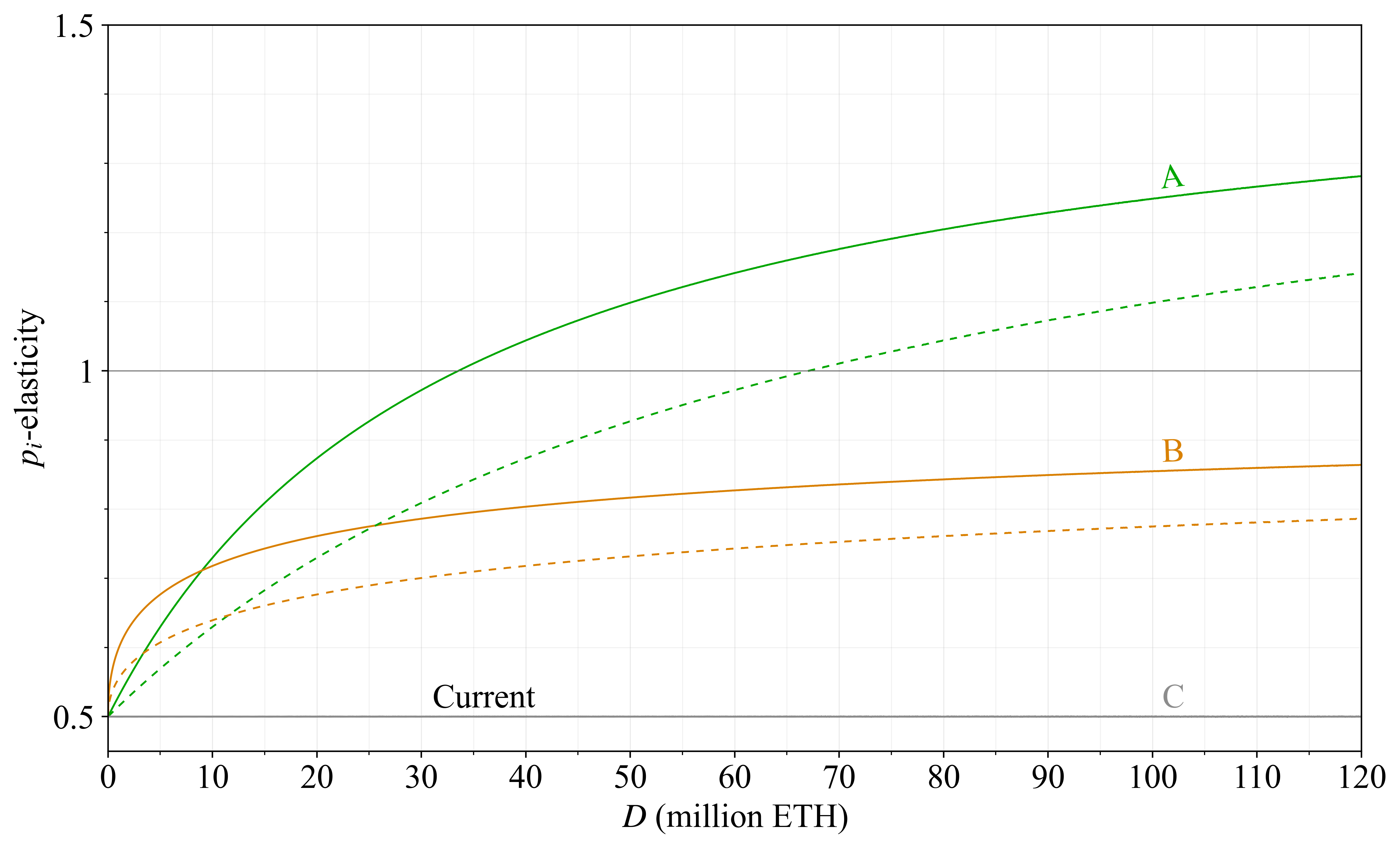
Figure 16. The point-wise negated inverse yield-elasticity of demand (p_i-elasticity) for the three reward curves examined in this post (lower is better).

The best defense against a minority discouragement attack is to have a well-balanced consensus mechanism. Ethereum should therefore in the future fix the current incentives that allow for infinite profit margins during an inactivity leak and for attacks with G=14. The second best defense, particularly useful against larger attackers (including majorities), is some form of social intervention, as discussed in Section 5.1. The prospect of social intervention can make the risk-reward ratio rather unfavorable for discouragement attacks. The immediate gain is rather low (in fact negative in most cases), and profits vary with frictions in the decision to stake or unstake. Finally, note that the prospect of being able to rely on social intervention in the first place could also depend on quantity staked, as outlined in Section 2.2, making the problem multi-dimensional. To balance the various aspects discussed in this subsection, it is desirable with a reward curve that gives appropriate guarantees for a sufficient quantity staked without providing excessive levels of issuance, and then reduces the incentive to stake across a broad range, for example by gradually attenuating issuance. This was one of the design rationales for the proposed reward curve (Option A).

5.4 Cartelization attacks

Cartelization attacks are hypothetical constructs related to and overlapping with discouragement attacks, that can differ in rationalization and execution. They will here be presented briefly. A cartelization attack consists of SSPs working together to try to reduce quantity staked both among themselves and others. When issuance increases with a reduction in quantity staked (p_i>1), all stakers could try to agree to reduce their stake, and everyone would be better off. This framing can provide a suitable backdrop for convincing the social layer to not interfere when a staking cartel tries to inhibit Ethereum’s permissionlessness. Ideally for the cartel, it would be able to rely on some permissioned revenue outside of the consensus mechanism that a majority can extract to incentivize initial participation. However, if insufficient (in particular once the yield has risen), the cartel could resort to more sinister actions within the consensus mechanism. The actions need not completely break consensus formation to be effective. Modest discouragement attacks against “strikebreakers” to ensure that such entities “stop reducing everyone’s rewards” could be sufficient.

If the reward curve is too deliberate about targeting some specific quantity staked, but still provides high issuance at lower quantities, then stakers may face a situation where cartelization and a reduction in quantity staked could lead to multiple times higher rewards for everyone. The proposed reward curve (Option A) incorporates a sufficiently small issuance reduction as D rises, so that the rationale for executing a cartelization attack is minimal/non-existent.

6. Conclusion and discussion

6.1 Factors influencing the optimal shape of the reward curve

Ethereum must weigh many factors when deciding on a reward curve. A low issuance level:

• improves aggregate utility by not compelling users to incur unnecessary costs. This is of fundamental importance, and it is the reason for why every ETH holder can benefit from a reduced issuance level.
• keeps the quantity staked moderate. This reduces:
  • the risks posed by a compromised social layer,
  • network externalities that entrench dominant SSPs,
  • economies of scale of dominant SSPs.

However, an excessively low issuance level might sideline solo (home) stakers down the line, if the yield is reduced so much that staking on a reasonably efficient setup becomes unprofitable. Retention of a viable proportion of solo stakers will hinge on the distribution of reservation yields among all stakers, accounting for scenarios where initial exogenous incentives for solo staking (e.g., airdrops) have dried out and initial hardware investments have reached their depreciation horizon.

From a security perspective, it is beneficial to keep the yield rather high at low quantities staked to ensure a sufficient quantity of stake and economic security. But to protect against discouragement attacks and cartelization attacks, it is also beneficial if issuance does not then fall too sharply at any point, i.e., it is best if the p_i-elasticity is kept rather moderate. This therefore also becomes a balancing act, where it is best that issuance is not too high and not too low at any deposit size.

Additional complexities arise from MEV captured by block proposers:

• It raises the expected yield, so a lower issuance is required to enforce the same quantity staked.
• But issuance cannot be reduced too much without compromising consensus incentives under the current specification. Resolutions such as a staking fee could further debilitate solo staking, relative to delegated staking.
• It raises variability in the expected equilibrium yield at a macro level, complicating the effort to achieve any specific desirable equilibrium.
• It raises variability in the expected yield of individual solo stakers, leading to some utility degradation if the issuance is set too low.

6.2 The optimal reward curve

6.2.1 Option A – the best alternative for Ethereum

The candidate reward curve, Option A, was designed to effectively moderate issuance while allowing Ethereum to retain proper consensus incentives and keep solo-staking variability acceptable. Section 2.1 highlighted the undeniable benefits of minimum viable issuance—the reduction in the implied cost to Ethereum’s users and the associated aggregate utility gain, which may very well make everyone better off under equilibrium. Section 2.2 further strengthened the case by deliberating on the clear benefits of a neutral social layer that can ensure that Ethereum operates under the intended consensus process. Option A will best attain these benefits, and it was in a previous study selected over even stricter issuance policies because of its balanced approach to various relevant trade-offs. It is not clear which issuance level that will maximize the proportion of solo stakers (and the outcome can vary with time scale considered), with arguments in both directions reviewed in Section 4.2. Importantly, a low quantity of stake is not strictly forced, ensuring that the cost of running a staking node will not be prohibitively high relative to the yield. This ultimately allows variety in preferences and circumstances between stakers to take a more central role in shaping the composition of the staking set. The proposed reward curve also ensures economic security in both the short run and long run while being sufficiently resilient against discouragement attacks and cartelization attacks, retaining an intact social layer by a gradual attenuation of issuance with modest p_i-elasticities.

Another benefit of Option A is its ease of interpretation: a single adjustable variable defines both the peak issuance point as well as the point where issuance is halved relative to the current reward curve. As noted in Section 2.3, compromising the predictive capacity of economic agents undermines welfare. It is also desirable to accommodates reevaluation against uncertain future stake growth and solo-staking retention scenarios, in particular in light of a potential future MEV-burn implementation. Therefore, a graduated reduction of issuance is preferable when possible, allowing for gradual adaptation.

In conclusion, the author believes that a holistic approach to issuance policy makes Option A—the candidate reward curve—the most suitable reward curve for Ethereum:

y_i=\frac{cF}{\sqrt{D}(1+D/k)}.

The full envisioned reduction constitutes k=2^{25}. In the author’s view, a graduated approach with k=2^{26} is preferable. This is still a sufficiently substantial improvement to warrant the multifaceted governance process associated with a change to issuance policy, and would position Ethereum much better going forward. From a security perspective, such a change would not pose risks, and Ethereum could thus proceed with it whenever the governance process has taken its course. The exact setting should be determined during that governance process, and will be based on circumstances that may evolve during the process. Alternatives such as setting k to 2^{25}, 2^{27} or 10^{8} cannot definitely be ruled out at this point.

6.2.2 Option C – the backup

The second best option is to reduce the base reward factor, i.e., Option C. Two things can be noted: (1) the consensus specification change is even more minimal, (2) the guaranteed yield for (solo) stakers is higher. Of course, to many, (2) would instead be considered a drawback, since it will lead to a higher equilibrium quantity of stake, making problematic outcomes in this regard much more likely as compared with Option A. Even if the endgame is Option A, the graduated first step can still be taken with Option C. But it would in the author’s be preferable to proceed with Option A, giving the community a clear path and roadmap. Option B, perhaps also with F=64, is a compromise between A and C, and can be called upon if agreement cannot be made between them.

6.3 The unknown endgame

The optimal “endgame” of Ethereum staking economics is at this point unknown, and will remain so, probably for at least another decade. It depends on many aspects that have currently not been settled, one of them being the specification of the endgame consensus mechanism itself.

There are however reasons to believe that the proposed reward curve can be viable for a long time, perhaps forever. For example, consider the scenario where the community feels that it is important to temper the quantity staked. The full reduction can then be implemented with k=2^{25} in the not-too-distant future, and kept when instigating MEV burn. The other two alternatives are to go back to k=2^{26} once MEV burn can be implemented, or to stop already at k=2^{26}: if MEV burn turns out to be viable and the community is satisfied with that as the second step. At k=2^{25} and with MEV burn, the staking yield would indeed become rather low (see the lime-colored curve in Figure 33 of this post). As an example, the issuance yield is 0.77 % at 60M ETH staked. When accounting for risks (slashing, smart contracts, governance, etc.), and other costs of staking, it seems rather unlikely that the quantity staked would be pushed above 60M ETH at such a low yield. Yet, even if this turns out to hold true, it should not be interpreted as arguing that the proposed reward curve necessarily must remain in place indefinitely—just that it seems rather suitable as an endgame and offers clear improvement relative to the current reward curve. The optimal quantity staked ultimately depends on the shape of the supply curve (representing possible attainable yield–quantity combinations), and how the relative importance of the various trade-offs that Ethereum balances will evolve in the future.

There is one thing that certainly remains for the endgame even after adopting the proposed reward curve. The long-run staking equilibrium under reward curves that adapt to D instead of d is ultimately also influenced by the circulating supply equilibrium, since the circulating supply will drift to balance supply, demand, and protocol income. Therefore, Ethereum should transition to using d in the equation for the reward curve, which can simply be done by swapping in the circulating supply, once it begins to be tracked.

The benefits of not issuing more tokens than what is strictly needed for security are indeed clear and substantial. Schwarz-Shilling and Dietrich present benefits and argue for an endgame of targeting a low quantity staked, potentially through economic capping (a yield that goes to negative infinity when too much ETH is staked). When it comes to solo staking, the analysis looks at a hypothetical scenario where the reservation yield is 1.5 % at 30M ETH staked and 2 % at 120M ETH staked. Under a flat supply curve with high reservation yields, stricter targeting (a steeper reward curve) at low quantities staked indeed seems rather straightforward. Solo staking will with such supply curves always be viable, regardless of the shape of the reward curve. Under the supply curve of Figure 12, a strict targeting approach could instead force outcomes that may be unfavorable to the composition of the staking set. Priors regarding the possible shapes of the supply curve here matter. Discouragement attacks and cartelization attacks become more viable with targeting approaches where the equilibrium p-elasticity is pushed up too high. To solo stakers, uncertainty itself regarding if the yield will go negative may make them hold off on investing in hardware. Indeed, certainty pertaining to either yield or quantity staked is always substituted via the shape of the reward curve. A flatter demand curve will smooth out fluctuations in yield, and can therefore decrease the equilibrium yield, ceteris paribus (at the same quantity staked), since economic agents may be willing to substitute lower variability for lower returns. But a steeper demand curve instead gives smaller fluctuations in quantity staked, and better assurances concerning its maximum level. The author has gradually changed position, from favoring strict deposit ratio targeting in 2021, to gradually focusing on targeting a desirable deposit ratio range (where the range of plausible equilibria can be rather broad to balance the trade-offs that exist), settling on the proposed reward curve as the correct mechanism for balancing current circumstances pertaining to MEV, with the implementation of MEV burn allowing the same reward curve to potentially transition into a viable endgame policy. Yet, it is important to remain open to changes when new information comes in over the next decade, updating priors, and reflecting on evolving trade-offs.

Finally note that there is no direct monetary purpose for staking when the endogenous yield is 0 or negative. Therefore, a negative issuance yield should only ever be needed when MEV or, e.g., rewards for preconfirmations befall the proposer. Thus, in all current scenarios with a negative issuance yield, unpooled solo stakers would be forced to accept negative payouts each epoch while waiting on proposer assignment, while delegating stakers could reap small positive rewards at a regular basis. When it comes to negative issuance yields, the most interesting option would be very gradual transitions at particularly undesirable levels of stake, e.g., subtracting (D/k)^p from current constructions for y_i, with p set to 0.5, 1 or 2. Reward curves asymptotically approaching 0 are in this case however perhaps more viable as an option. The optimal shape will ultimately depend on how the consensus mechanism itself develops (e.g., the role of solo stakers). Constructions with an infinitely negative issuance yield (which may technically be unreachable due to the churn limit) will however bring even more uncertainty to stakers and may bring unneeded complexity into the protocol design space.

Adding the dimension of time to the dimension of quantity is also worthy of consideration. Under a time–quantity policy, the reward curve is kept moderate in terms of elasticity, but the whole curve is allowed to gradually adapt to changes in the supply curve, implied by the equilibrium. Thus, under the proposed reward curve, k drifts when d ventures off desirable levels, with effects taking place at a time scale of decades. This would allow Ethereum to account for the supply curve when setting the reward curve. The mechanism would smooth out fluctuations in yield, and the delayed adjustment could make some discouragement attacks and cartelization attacks less attractive. Certain limits could be placed on how small k can become with this strategy, to avoid idiosyncratic outcomes. There is also a distinction here between automatically increasing the yield (opening up for discouragement attacks) and decreasing it (opening up for the familiar issues associated with low yields). Interestingly, while the protocol may not be able to determine who is at fault in a discouragement attack, it can still determine that it is in fact under attack, providing an avenue for safeguards through conditional logic.

6.4 The proportion that matters to ETH holders

The insights presented in Sections 2.1, 2.2, and 4 have implications for Ethereum’s users, irrespective of if they hold significant amounts of ETH. Having a viable social layer—uncorrupted by any SSP—ultimately matters to credible neutrality. Having solo stakers matters, and having many viable options for delegated staking matters. These things also matter specifically to the ETH token holder. It is ultimately not the “proportional yield”, but rather the proportion of the world economy powered by Ethereum that will affect the ETH token holder the most, including the staker. If an issuance policy degrades Ethereum, there is little point in having maximized y_p, certainly not to users that do not hold ETH, and not even to ETH token holders, because the native token of a blockchain that has been degraded is not as valuable. The real “real yield” incorporates the change in value of the underlying ETH—including any staking yield—relative to a relevant consumer price index. However, it just so happens that it is indeed very useful to have sound native money in an economic system. And it so happens that the best sound money will not encumber its users to research the reliability of various SSPs, track staking income and see it taxed, or risk being wiped out in a slashing event or other failure.

6.5 A note on bounded rationality and yield

The notion of bounded rationality helps to explain why some users may prefer a scenario with lower y_p, where the yield is raised but the supply inflation rate (which users have a harder time to track) rises even more. Behavioral economics can be helpful in this way for explaining why some economic agents act irrationally, perhaps for lack of education or time to deliberate on a topic. Recently, a twisted argument relying on bounded rationality has appeared in the writings of several representatives of SSPs or investors thereof. In essence, proponents suggest that Ethereum should harness people’s bounded understanding of yield, and keep it high to trick users into thinking that they gain something, when they do in fact not. Instead of educating people on these matters, user utility should be degraded for some short-term gain, which is unlikely to materialize. Such strategies must be avoided.

6.6 Next step

The author hopes that this post has convinced the community of the benefits of adjusting the issuance policy, and is available for any questions you may have. The post will act as the long-form reference for the EIP on the proposed reward curve—Option A. Making the full reduction in a single hard fork seems unadvisable, and the outlined graduated approach favorable. That first step brings essentially no downsides, will improve Ethereum substantially, and if not the final step it is still a step in the right direction.

[themandalore]

Super cool!

I think from your post, it seems like you’re saying: “current rates are too high and we’re going to have 100% staked before we know it, so let’s lower it now so we have time to reexamine”

My question is, why not make it more extreme favoring the current set then? Under these curves (that don’t go negative), exogenous rewards could still push it way too high. Or is the idea just to get people used to the idea of tweaking it to target an amount staked?

[aelowsson]

@themandalore

I think from your post, it seems like you’re saying: “current rates are too high and we’re going to have 100% staked before we know it, so let’s lower it now so we have time to reexamine”

I actually do not think we will have 100 % before we know it. As I outline with the hypothetical supply curves, I think a reasonable expectation is 50M ETH staked two years from now. It may seem as if this then would indicate that there is no harm in waiting, but that is incorrect if you agree with the arguments in Section 2.1. It is also notable that under such a supply curve, the effect on solo stakers with worse economies of scale would be the least harmful. Quick changes are always negative, and it is important to review feedback from the community around that (this is also why I favor a graduated approach). But I think that since a graduated approach is so clearly beneficial to Ethereum’s users, it is my job to suggest taking a first step out of two as soon as this is possible. That is simply in recognition of the fact that it would improve Ethereum. This does not mean that there should be a strong push for a quick change under contentious circumstances. I think it is perfectly reasonable to review feedback and let the community digest the ideas in proper time.

@themandalore

My question is, why not make it more extreme favoring the current set then?

It is not possible to favor the current set specifically. The current set might leave (at least when their hardware must be upgraded), and be replaced by a new set of stakers of equal size with better economies of scale.

@themandalore

Under these curves (that don’t go negative), exogenous rewards could still push it way too high. Or is the idea just to get people used to the idea of tweaking it to target an amount staked?

The idea is as you say to reexamine how things evolve, but the idea is not specifically to do any more tweaking after reaching k=2^{25}. One way to frame it is that the reward curve offers a yield across a broad range as a way to avoid extreme outcomes, either pertaining to yield or quantity staked.

[Chawbow]

This post was flagged by the community and is temporarily hidden.

[Mingo-ETH]

This post was flagged by the community and is temporarily hidden.