Properties of issuance level: consensus incentives and variability across potential reward curves
Thanks to Barnabé Monnot, Francesco D’Amato, Caspar Schwarz-Schilling, Thomas Thiery, Davide Crapis, Julian Ma, Vitalik Buterin, Justin Drake and Ansgar Dietrichs for review and/or fruitful discussions. Thanks also to Flashbots for providing the data used in the analysis.
This post is also available in a more compact format as a thread, but Section 5 offers several additions.
1. Introduction
1.1 Background
Ethereum’s stakers started to receive execution layer rewards with The Merge and liquidity improved when withdrawals were enabled with Shapella. Both upgrades have served to push up the equilibrium quantity of stake. The resulting increase in gossip messaging and to the Beacon state size puts strain on the consensus layer. An increase in staking deposits is furthermore associated with an increase in issuance of new tokens under the current reward curve, bringing an inflationary pressure on regular users who rely on ETH. Ethereum issues ETH to stakers to incentivize them to stake and secure the blockchain. But raising the issuance level if no further stake is needed—and even degrades both the consensus network and economics—is arguably not beneficial. The amount of stake that Ethereum needs to remain secure is a subject of active research and discussion, where many developers now argue that it is reasonable to moderate the growth. In preparation for such an effort, this post will analyze the effect of issuance level on consensus incentives and reward variability across potential reward curves.
1.2 Security and deposit size
The relationship between the staking deposit size D and Ethereum’s security level is not trivial to characterize. On the one hand, we may focus on the value slashed in an attack. Since one million (M) ETH is worth around 2.2 billion dollars today, the cost of attacking Ethereum using some critical proportion of D (which is currently 29M ETH), becomes very high under the threat of slashing. But a higher deposit size also provides Sybil resistance to more subtle forms of degradation to the consensus mechanism that may not immediately lead to slashing (e.g., short reorgs). Notably, the 14M ETH securing Ethereum at The Merge was found sufficiently secure by the ecosystem at the time, in a way acting as a “revealed preference” under those prevailing circumstances. In any case, there comes a point where the marginal increase in security from adding another validator brings less utility than the utility loss to users. A level of D=2^{25} ETH (33.6M ETH) has been used as a reference point of when network conditions (and economics) start to degrade. Drake expanded on his reasons for supporting a target of 30M ETH in a recent AMA. This active area of research is related to the concept of “minimum viable issuance”.
1.3 Minimum viable issuance
An ideal deposit size will satisfy minimum viable issuance, the idea that Ethereum should not issue more tokens than what is strictly needed for security. Excessive issuance—which is always an inflation tax on users—forces everyone to expend resources staking, or to face a principal–agent problem as a delegating staker, lest they want their ETH savings eroded. This degrades utility in aggregate. Staking income is also taxed in many jurisdictions, whereas circulating supply deflation is not. From a macro perspective, Ethereum avoids a scenario where a staking service provider (SSP) can come to dominate not only in terms of staked ETH under its control, but also in terms of the total circulating supply, making its issued liquid staking token (LST) a novel stratum for cartelization. A concern is that a majority of Ethereum’s users will be economically entangled with one or a few for-profit SSPs through its issued LST. In the case of a mistake or misdeed by the SSP, Ethereum’s social layer may then waver on its commitment to the underlying intended consensus process. It is arguably preferable to see Ethereum’s native token permeate and bind together the extended ecosystem (including rollups) instead of a derivative of it.
1.4 Consensus incentives
Ethereum’s consensus mechanism relies on a collection of micro incentives to ensure that validators perform their tasks correctly. The attester is rewarded for voting on a correct source and target checkpoint for Casper FFG, as well as the head block within LMD-GHOST. A missing/late or incorrect Casper FFG vote instead results in a penalty. The proposer attains 1/7 of the rewards given to attesters for including the attestations in the proposed block. The magnitudes of these micro incentives (including penalties) are ultimately regulated by the issuance level. This differs from the MEV and priority fees that the proposer also receives, which are unrelated to issuance policy. An equilibrium enforced through a reduction in issuance can unbalance the economic forces, rendering the micro incentives ineffective. Solo stakers would also be negatively affected by the increase in reward variability. Maintaining correct incentives as the issuance level and deposit size change is important.
1.5 Purpose and main questions
To what extent can Ethereum stop issuing more tokens than what is needed for security? Can we reduce issuance while still retaining consensus stability, proper incentives, and acceptable conditions for solo staking? Can we adopt a reward curve that lets the issuance yield go negative past some specific staking deposit size D, or target some specific desirable D by simply adapting the yield to enforce it? Otherwise, should a more moderate approach be adopted? This post will take a closer look at these questions and review features of staking economics that affect consensus incentives and reward variability—including how they vary across deposit size. The analysis shows the benefit of a moderately falling issuance as the deposit size rises above target levels, with relevant candidate reward curves evaluated in Section 5.
2. Equilibrium staking
2.1 Supply and demand
The base reward factor F is the parameter that directly adjusts the issuance level under the current reward curve, affecting all consensus rewards and penalties. Ethereum provides an issuance yield under idealized performance of y_i = \frac{cF}{\sqrt{D}}, where F=64 and the constant c\approx2.6. The total yield provided by the protocol to stakers implies its demand for stake and it is
where y_v is the yield from realized extractable value (REV). The REV is the value that stakers receive from priority fees and MEV after builders take their cut. Define the yearly aggregate REV as V (currently around 300k ETH). The expected yield from REV then becomes y_v=V/D. Going forward, the post will sometimes use overline when referring specifically to the demand curve, if needed for clarity (thus \overline{y}=y_i+y_v), and underline \underline{y} for the supply curve.
Note that the demand curve formed through \overline{y} is the “endogenous yield” derived exclusively from staked participation in the consensus process. The yield from DeFi (including “restaking”) that is exogenous to staking y_c, is not part of \overline{y}; it can under competitive equilibrium also be derived by non-stakers. It is convenient to separate \overline{y} and y_c in the analysis, to properly model what happens as \overline{y} falls towards zero. At that point, there will be no point in staking. Any yield derived outside of the consensus mechanism from staked ETH will also be possible to derive via non-staked ETH. For example, it will be better to “restake” WETH. Any DeFi service that fails to serve non-staked ETH will be outcompeted. This means that Ethereum must always offer a positive endogenous yield \overline{y}. This is a nice assurance to Ethereum’s stakers. This post will go a step further, and ascertain that y_i specifically also must be kept well above zero under the current version of the consensus mechanism (as an aside, if the REV is burned, y_i will also remain above 0, since there once again will be no point in staking if y_i=0).
Generally, y_c should be higher for non-stakers than stakers, because collateral that cannot simply evaporate is more reliable and valuable. Contemplate for example the effect that a majority client bug could have on an actively validated service collateralized solely by staked ETH. However, y_c can still incentivize users to supply stake at a lower staking yield, as long as the staking yield more than compensates for the staked ETH’s degradation as collateral. For example, say that an agent is willing to own and lock up ETH if the total acquired yield (including y_c) is over 0.04 (disregarding costs/risks for simplicity). Define y_c' as the yield from collateralizing non-staked ETH. If y+y_c > 0.04 and y+y_c > y_c', the agent will decide to stake ETH. Thus, if y_c = 0.01 and y_c'=0.02, the requirement is y> 0.03 for the agent to stake. But if y_c = 0.02 and y_c'=0.03 the requirement is only y> 0.02.
The shape of the supply curve is unknown and affected by many variables. Plots will be provided in this post covering a broader range so that different assumptions can be mapped to various outcomes. As a guideline, two supply curves will be included in the plots. The equation used for the (inverse) supply curve is
using the deposit ratio d (the fraction of the around 120M circulating ETH that is staked), with k=1/2, c_2=0.003. The first term c_1d^{1/2} gives the curves a yield elasticity of supply of around 2 in the middle range. The term \frac{c_2d}{1-d} captures the notion that the final fraction of the circulating supply may not be staked in the medium run until the yield becomes very high. The opposite, a downward-sloping supply curve due to network effects of LSTs, seems a bit far-fetched. The variable c_1 is set so that \underline{y} reaches some specific deposit size at some plausible yield. In this post, the two curves were set to reach D= 25M at y=0.025 and y=0.02 respectively. The upper curve could for example represent the supply curve underpinning an equilibrium within a year or two, whereas the lower curve could be the supply curve after a few years of improvements to the the staking experience and better financial integrations.
This post tracks supply and demand across D (specifically, it does not track the circulating supply and its effect on d), which means that it deals with medium-run staking equilibria. The long-run staking equilibrium under reward curves that adapt to D is ultimately also influenced by the circulating supply equilibrium, since the circulating supply will drift to balance supply, demand, and protocol income.
2.2 Influence of F on the equilibrium
Figure 1 plots a hypothetical medium-run equilibrium staking. The colormap and y-axis both capture y, with the colormap restricted to F \in [0, 75]. At equilibrium, the demand curve will intersect the supply curve. Hypothetical equilibria under the current issuance policy (F=64) at the prevailing level of REV are indicated by blue circles. The hypothetical equilibria if issuance is halved (F=32) are indicated by blue squares. Such a reduction brings the deposit size closer to a previously suggested desirable range in between the dashed blue lines. The left dashed blue line indicates 14M ETH and the right dashed line indicates 33.6M ETH.
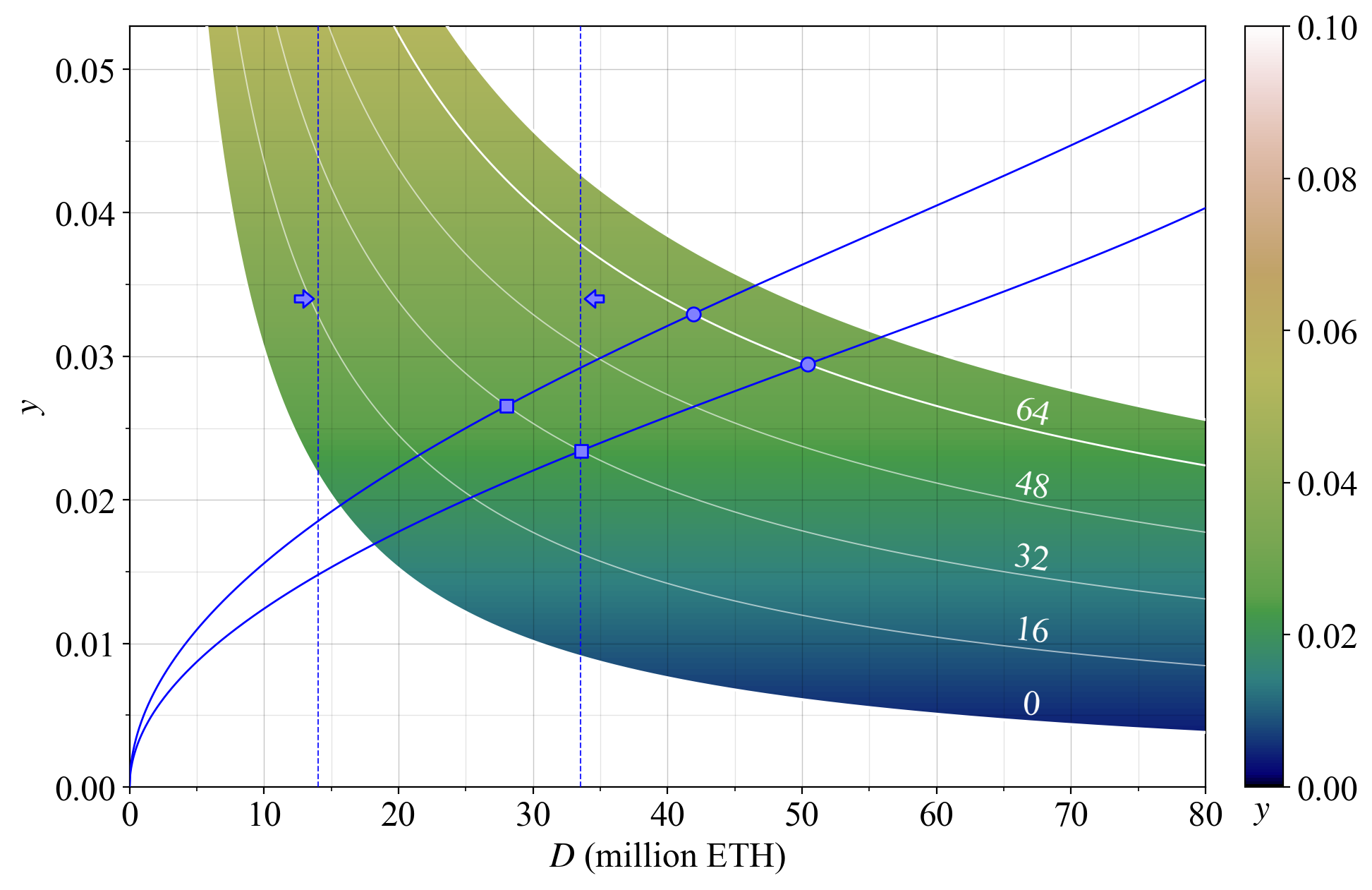
Figure 1. Medium-run staking equilibrium between the supply of stake (blue hypothetical supply curves) and demand for stake (white reward curves at various settings for F under the current level of REV). The y-axis represents staking yield and the x-axis deposited stake. It has been suggested that Ethereum should strive for an equilibrium between the vertical dashed blue lines indicated by arrows.
It is not possible to ascertain the exact effect of a reduction in F, but we can be rather certain that the yield elasticity of supply for the medium run is not 0 (a vertical supply curve). Reducing F will therefore always reduce the quantity of stake, ceteris paribus. Figure 2 shows that the full reduction in yield from a change in F (white downwards arrow) will not remain at the new equilibrium, because some stakers will presumably leave (blue leftwards arrow), bringing the yield for remaining stakers back up a bit (white leftwards arrow).
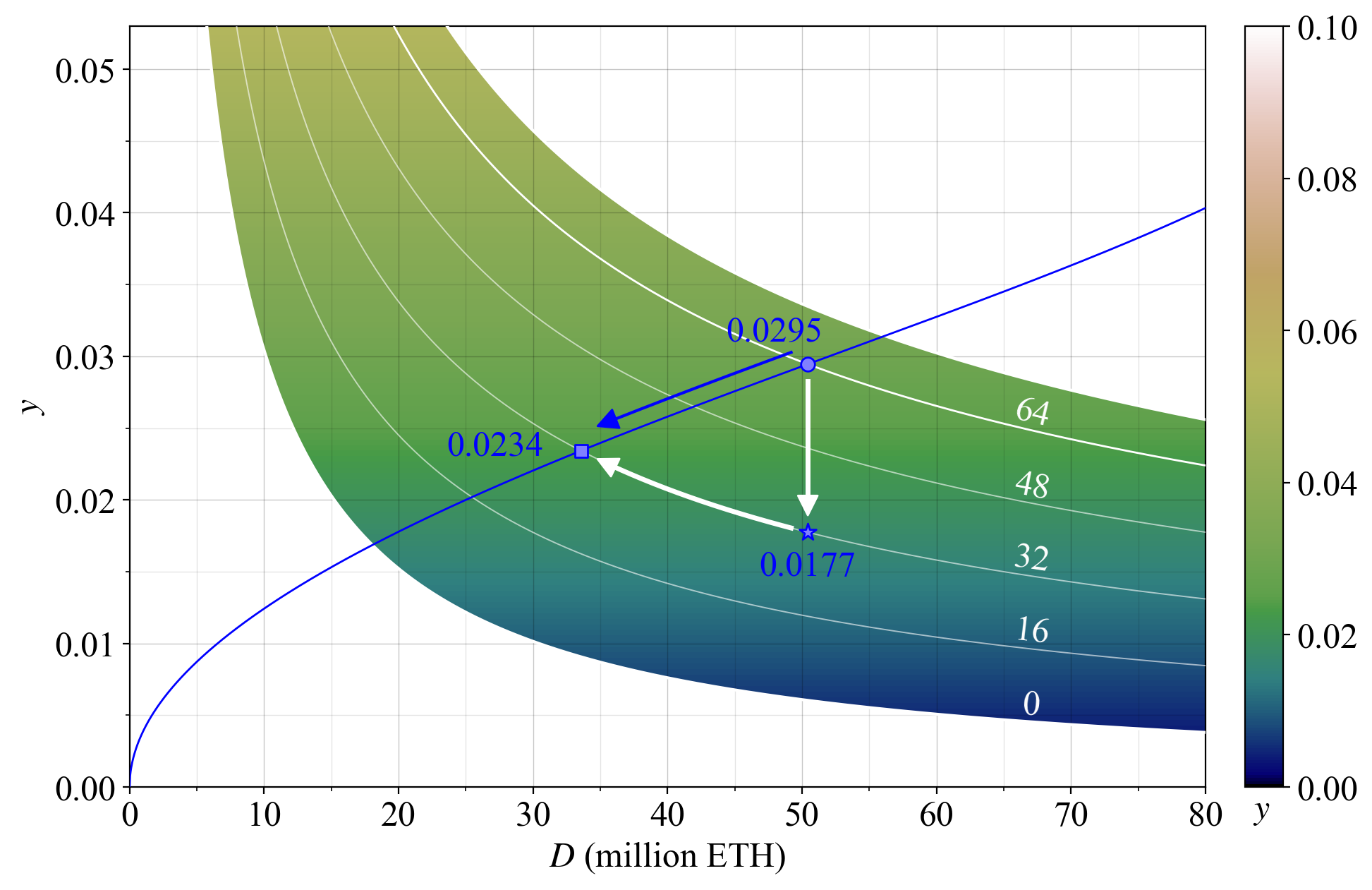
Figure 2. Hypothetical effect of a reduction to F from 64 to 32. The equilibrium yield initially falls from 2.95 % to 1.77 %, but then comes back up to 2.34 % as some stakers leave. Around half of the initially lost yield is thus recouped with this supply and demand curve.
How will this dynamic affect the solo staker and delegating staker? The outcome over shorter time horizons will depend on variations in cost structures and frictions affecting the decision to stake or de-stake. A solo staker who will not buy new hardware at some low yield may still stake over the lifetime of their current hardware. Delegating stakers dissatisfied with the yield may keep their savings in the LST until the next time they wish to spend their money, or leave directly. Solo stakers’ upfront costs and illiquidity presumably give them a lower yield elasticity of supply in the short run. This is comforting, because a temporarily lower-than-equilibrium yield (if F is reduced in a hard fork) may not push them out forever.
It seems likely that the supply curve will gradually shift downwards over time as the staking experience simplifies and DeFi integrations improve. The outlined dynamic in Figure 2 may therefore not fully materialize, as a lowering supply curve can nullify any de-staking process. The equilibrium quantity of stake will however still be lower with a reduction in F than if F is kept fixed. We must evaluate each possible outcome at the medium-run equilibrium. The effect of a gradually lowering supply curve is a gradually increasing deposit size.
Figure 3 has F on the y-axis (thus essentially the demand curve) instead of yield. You may think of it as dragging down and straightening the bent colormap in Figure 1 such that it becomes a rectangle. The colors encode the same yield as previously (also indicated by black lines). This viewpoint is convenient as the post now further explores the effect of a change to the issuance level. Both alternative graphs will often be provided to the reader and the same two supply curves indicated as guidelines.
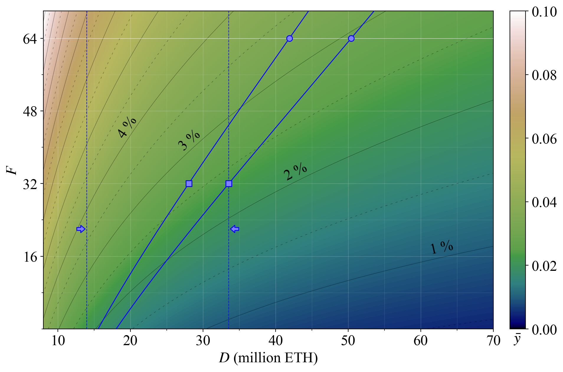
Figure 3. The same staking equilibrium as in Figure 1, but this time with the base reward factor F (regulating the demand curve) on the y-axis. The colormap still encodes staking yield.
3. Consensus incentives
When contemplating a change to the issuance policy, it is important to consider the effects on consensus stability, in particular how incentives may change for different consensus roles that validators will be assigned to. Figure 4 shows the proportion of the yield stemming from issuance at various settings for any specific base reward factor F. Naturally, the lower F is set, the lower the proportion of rewards that come from issuance. Right now at the prevailing level of REV, more than 2/3 of the yield comes from issuance. Since y_v falls by the reciprocal of D, whereas y_i falls by the reciprocal of \sqrt{D} under the current reward curve, a higher proportion of the yield will stem from issuance at a higher D.
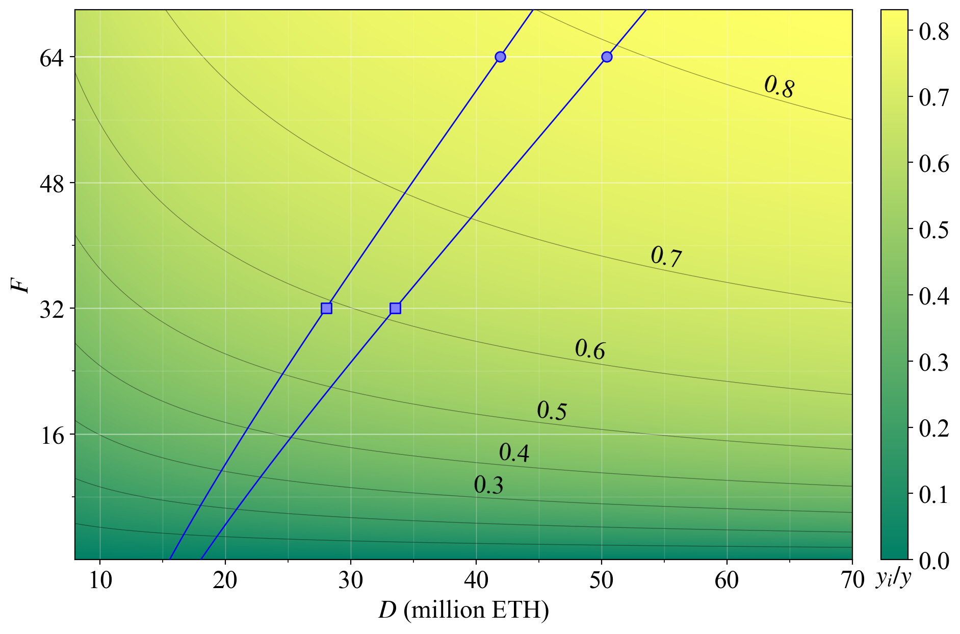
Figure 4. The proportion of staking yield derived from issuance (as opposed to REV), with F on the y-axis and D on the x-axis.
Figure 5 instead shows the yield that comes from attester duties (y_a) in proportion to all staking yield y_a/y (note that the measure thus incorporates the small yield from sync-committtee attestations in y_a, although these attestations functionally differ somewhat). Since the proposer gets 1/8 of the issued rewards, the reported proportion in y_a/y is lower than in y_i/y. If F is reduced to 32, almost half the rewards will come from the sparse chances of proposing a block. There is no well-defined proportion of y that must be provided for attester duties, but higher is generally better. This post will use y_a/y>1/2 as a guideline of a more healthy situation, y_a/y<1/3 as unhealthy, and y_a/y<1/4 as an outcome to be avoided. These guidelines are rather arbitrary, and a good subject for further research.
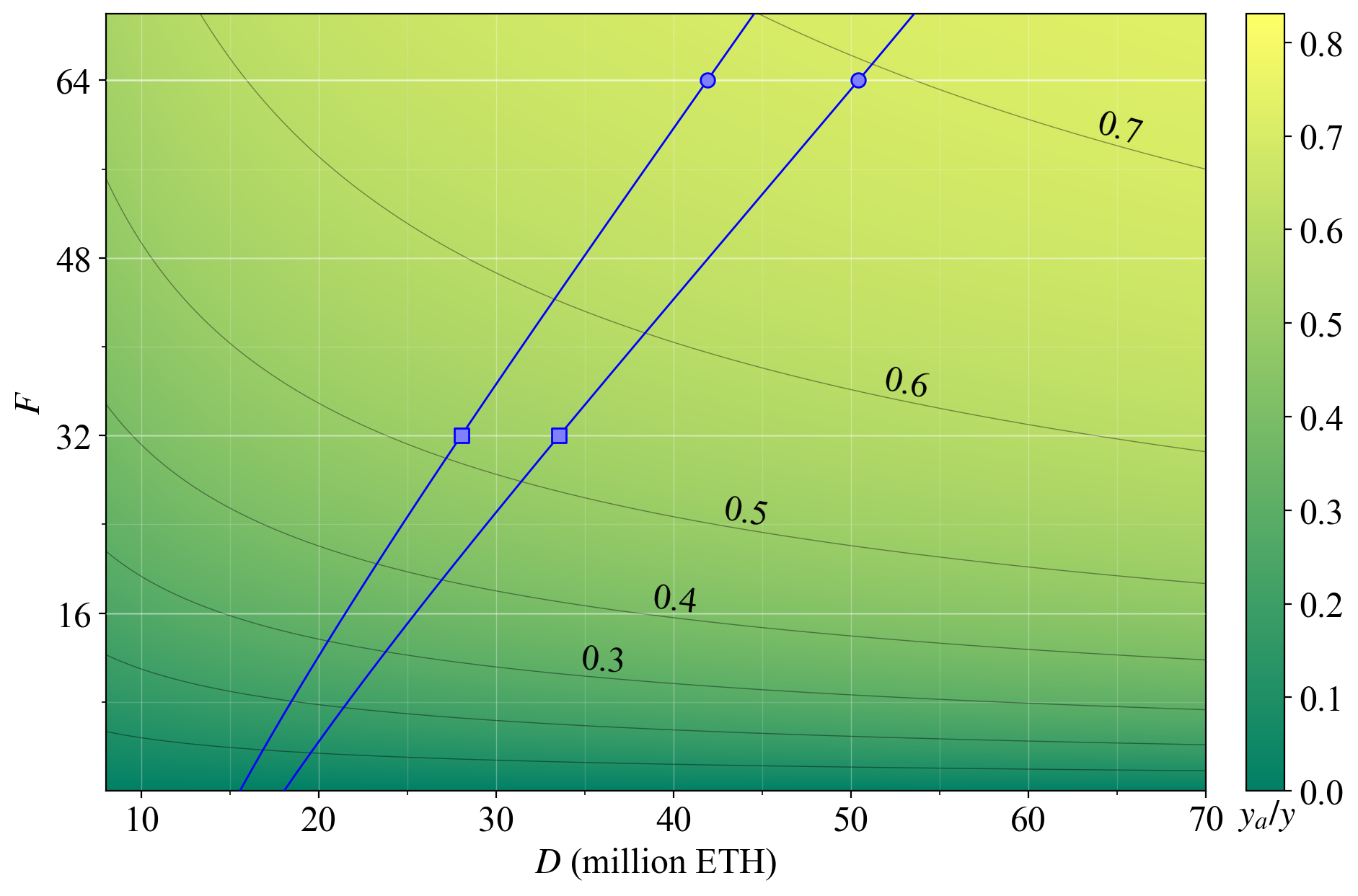
Figure 5. The proportion of staking yield derived from accurately performing attester duties (as opposed to proposer duties), with F on the y-axis and D on the x-axis.
When y_i/y and y_a/y fall too low, the consensus mechanism breaks down. Consensus rewards and penalties stop providing correct incentives for stakers. Honest attestation is less compelling. The only thing that matters is to collect REV and to not get slashed. Ignoring attester duties comes at little to no cost as long as the inactivity leak is not triggered, and instigating reorgs will be more tempting. If REV rises relative to the proposer reward, timing games also become relatively more attractive.
Moving back to having staking yield on the y-axis in Figure 6 gives another perspective on how various hypothetical changes to issuance policy may affect the proportion of rewards awarded for attestation. This time, the x-axis extends across the full circulating supply.
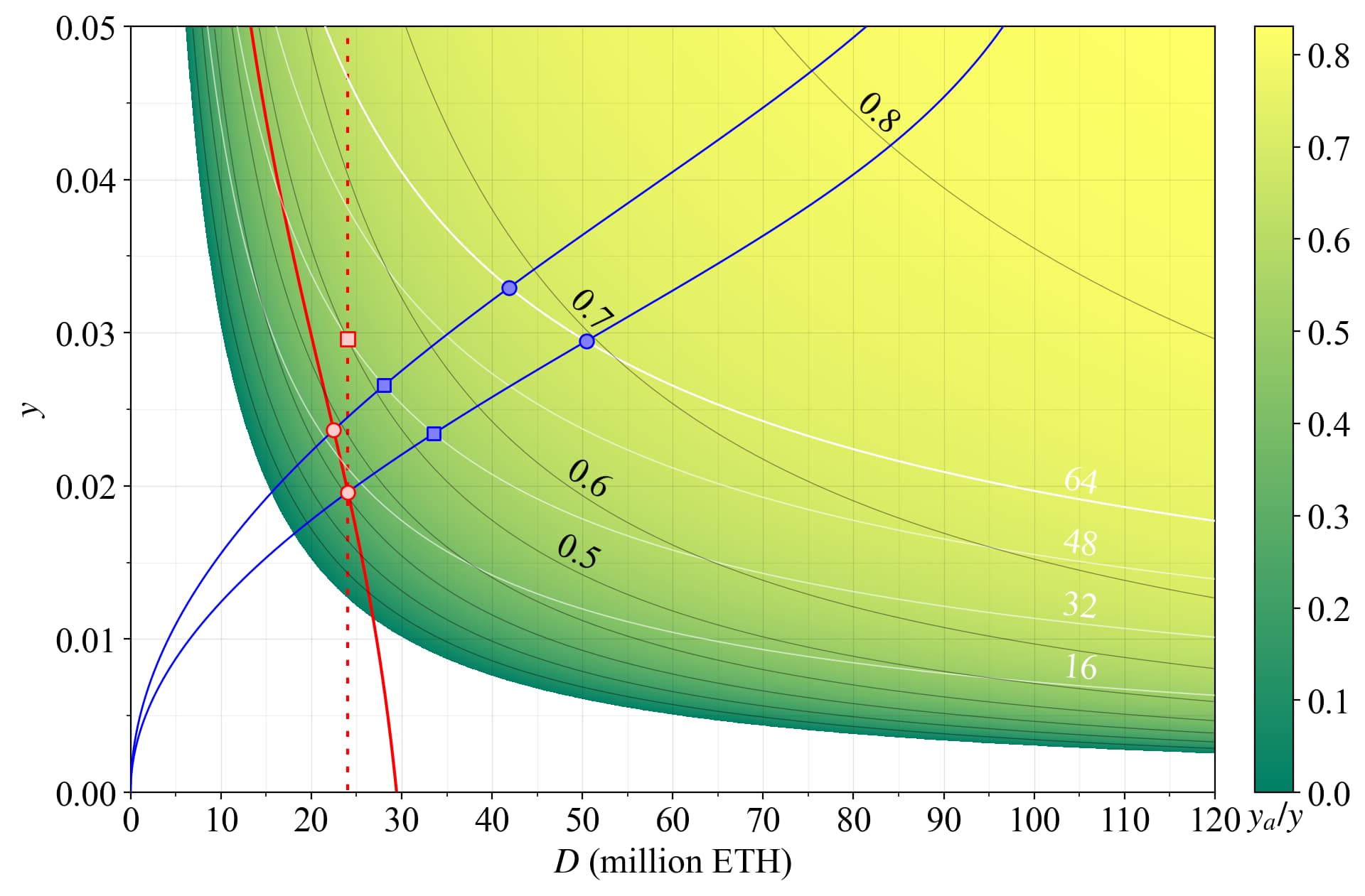
Figure 6. The proportion of staking yield derived from accurately performing attester duties (as opposed to proposer duties), with y on the y-axis and D on the x-axis. The red curve represents a previously proposed reward curve, and the dashed red line is the implied reward curve of targeting a specific quantity of stake.
In red, we contemplate the various stricter issuance policies that can be attempted, and the adverse effects they may bring before MEV burn is in place. For example, to target D =\, 24M ETH (dashed red line) while keeping y_a/y>0.5, the yield must be around 3 % (red square). This seems unreasonably high given that the supply curve slopes upwards. Therefore, to enforce D =\, 24M ETH, an even lower proportion of rewards must be given for attester duties. Indeed, even if these duties are not given any issuance rewards at all, an equilibrium may still not be achieved. An equilibrium where the issuance yield is “negative” is manifested by the white region of the figure. This could be the only possible equilibrium if the supply curve over time drifts lower—which seems like a very reasonable assumption—or simply because of a not particularly unlikely rise in REV.
The same type of problem can be encountered when adopting a reward curve that goes negative to enforce a deposit size below some specific level. The red line indicates the reward curve previously suggested by Buterin. At many reasonable equilibria with such strict reward curves, the rewards for attester duties will be very low (red circles), or non-existent. The breakdown of the consensus mechanism is then complete.
As previously outlined, when D rises, the white region representing y_v becomes smaller and smaller. This happens because y_v falls by the reciprocal with a rise in D. At 120M ETH staked, y_v is just 0.25 %. A quadrupling of REV would only lead to y_v=0.01 at 120M ETH staked, but to the rather imposing y_v=0.04 at 30M ETH staked. The important notion to take away from this particular discussion is that the lower the deposit size that Ethereum tries to enforce a staking equilibrium at before MEV burn, the more influential REV is going to be.
Some of the issues of a lower issuance here outlined can be remedied by taking out a staking fee each epoch and increasing the base reward correspondingly. To prevent consensus breakdown, the fee must be introduced already at positive yields, for example when y_a/y<0.5 or y_a/y<0.33. However, introducing a fee challenges long-standing tenets promoted to solo stakers (“you can go offline X % of the time and still break even”, etc.). Trying to push through these far-reaching changes when MEV burn eventually can make them obsolete therefore seems undesirable. Furthermore, a staking fee will not resolve other issues of a very low issuance, such as a rise in the relative and equilibrium variability in rewards for stakers that do not pool their MEV income.
4. Variability in rewards for solo stakers
The variability in rewards is higher for solo stakers than delegating stakers under the current consensus mechanism, because delegating stakers can in a frictionless manner rely on pooling of rewards from a large number of validators. This affects solo stakers negatively. A change in issuance policy could further widen the gap in variability, and it is therefore necessary to model that. The most prominent research on reward variability has been done by Pintail, with analysis up until and just after The Merge. The reader is also encouraged to study writings on this matter by Edgington.
4.1 Model
This post models variability for solo validators over one year in a rather simple fashion, with the distribution in proposer and sync-committee duties assigned according to the probabilities given from the consensus spec at each modeled deposit size. The focus is on the greatest source of variability, namely that of variation in REV. To this end, block proposers are assigned REV using sampling with replacement from the roughly 2.7 million block-level sample points provided by Flashbots. The probability density function (PDF) in Figure 7 of the REV in Ethereum shows a positive skew, with a mode of around 0.025. The mean of around 0.12, indicated by a dashed vertical line, is higher due to the occasional blocks with very high REV.
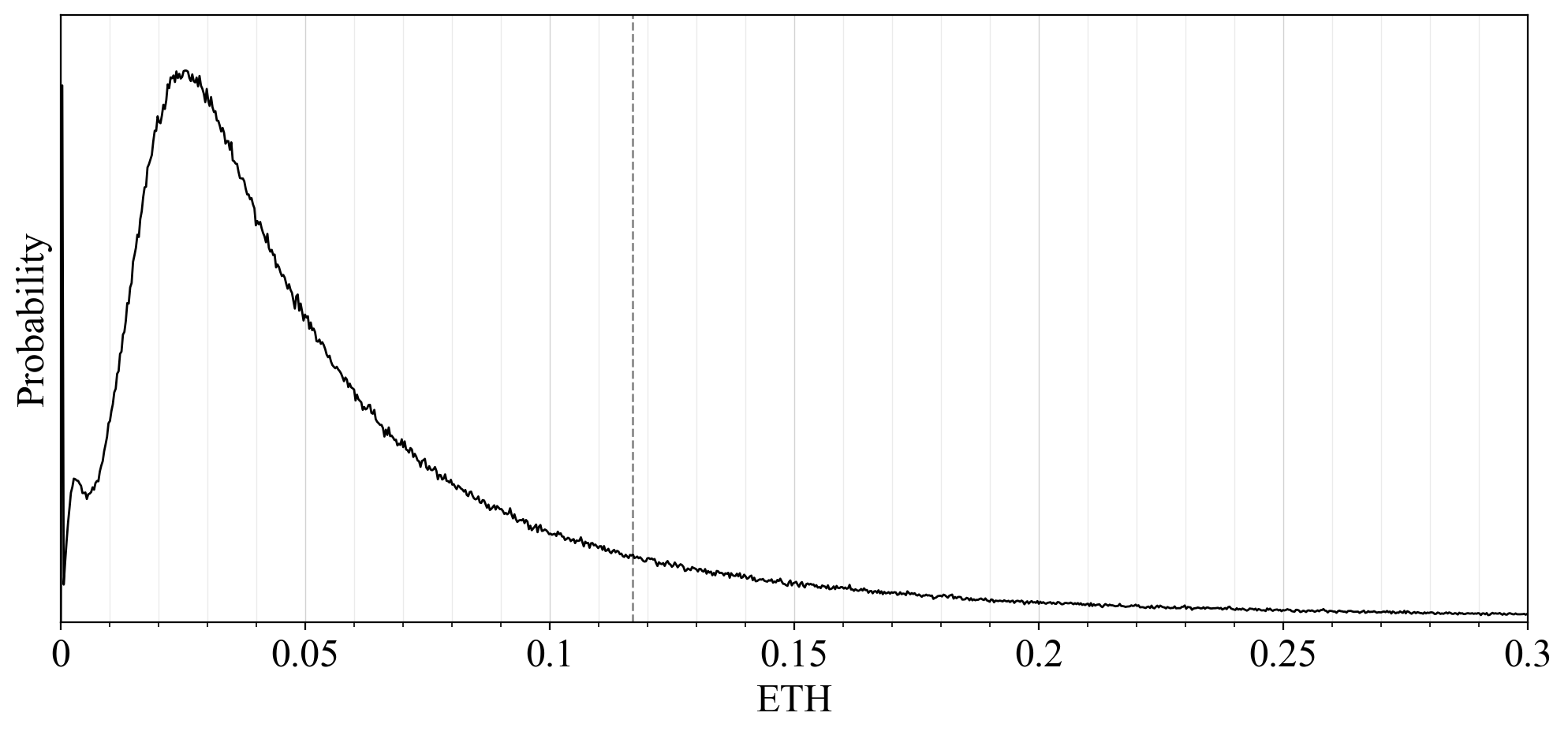
Figure 7. A PDF of Realized extractable value (REV) in 2.7 million blocks of Ethereum since The Merge.
To discern more details, the cumulative distribution function (CDF) is plotted in Figure 8 with a log-scaled x-axis and a logit-scaled y-axis. The median REV is around 0.045 ETH and less than 20 % of the slots are above the mean. The “median block” will thus still provide higher rewards for attesters than the proposer even as y_a/y=0.5. But the assertion in Section 3 is not specifically that all blocks provide the proposer with more value when y_a/y<0.5. Instead, it is rather that of generally misaligned incentives and systemic risk, which Ethereum is better off avoiding if possible.
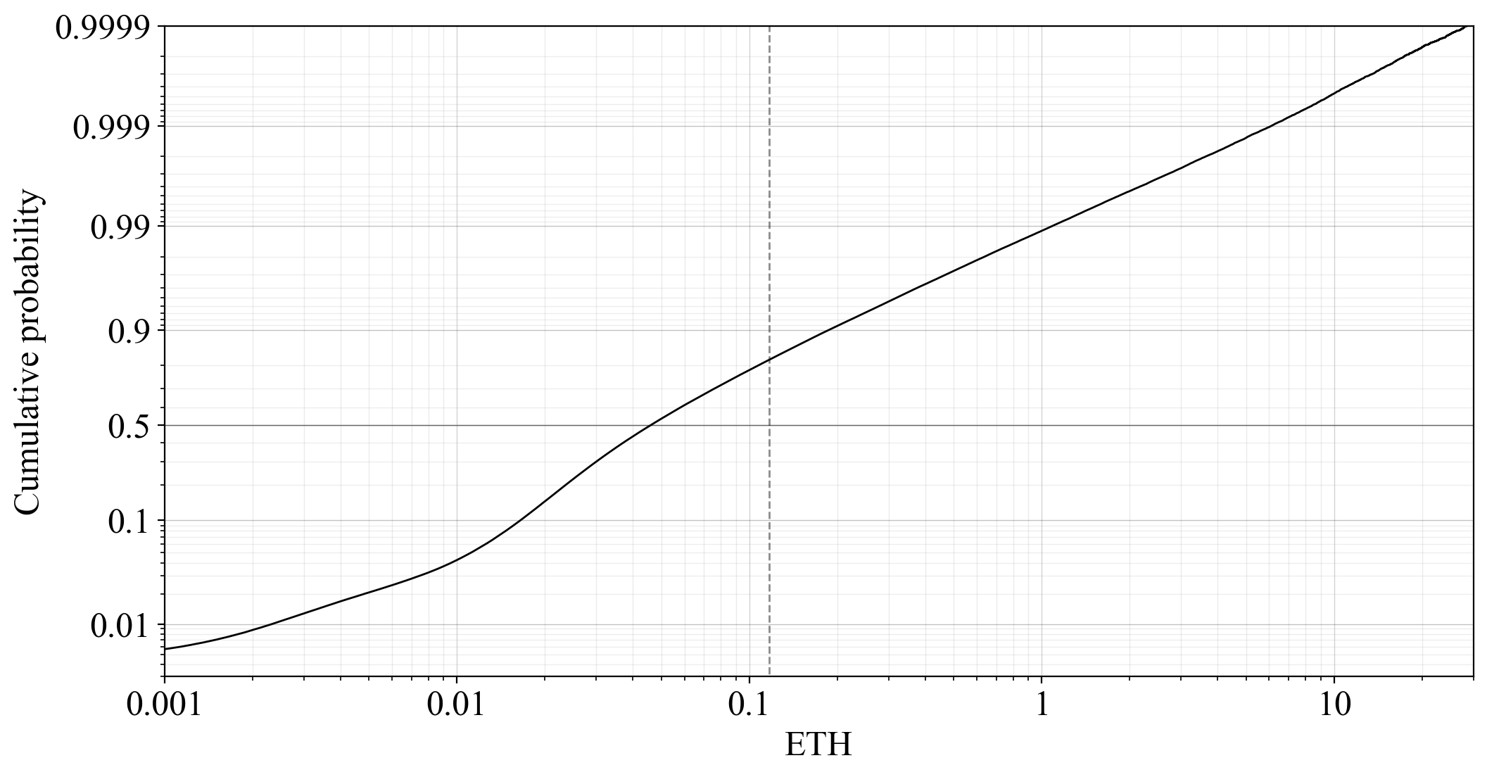
Figure 8. A CDF of Realized extractable value (REV) in 2.7 million blocks of Ethereum since The Merge. Note that the x-axis is log-scaled and the y-axis logit-scaled.
Blocks have been missed with a probability of around 0.96 % since The Merge, a condition that is also included in the model. Missed sync-committee assignments are not precisely modeled and instead assigned to have the same probability as missed blocks. It is presumably a lot less common to fully miss the sync-committee assignment (which spans over more than a day), and much more likely to partially miss it, but modeling this exactly is beyond the scope of this post. Notably, blocks are to a higher proportion missed by solo stakers than professional stakers, something that further degrades conditions for solo stakers when y_i is reduced relative to y_v. This specific feature is not included in the model. Finally, attesters are assumed to perform their duties correctly and are set to receive the full rewards (a slight overestimate). Variation in attestation accuracy will produce much less variability than selection for special duties such as block proposals, so it is less relevant to the analysis.
4.2 Effect of pooling
Figure 9 shows the influence of pooling on variability in staking yield at the current deposit size of D= 29M ETH, using CDFs of different pool sizes. Annualized validator rewards were simulated 30M times, sampling REV with replacement (s. w. r.). Pools were created from these distributions, also s. w. r. 30M times. As evident, variability is gradually reduced with more staked ETH (the curve becomes steeper). A solo staker running 2 or 5 validators can already reduce variance quite a bit; a small pool managing a couple of thousand ETH will still not be able to fully remove variance; etc.
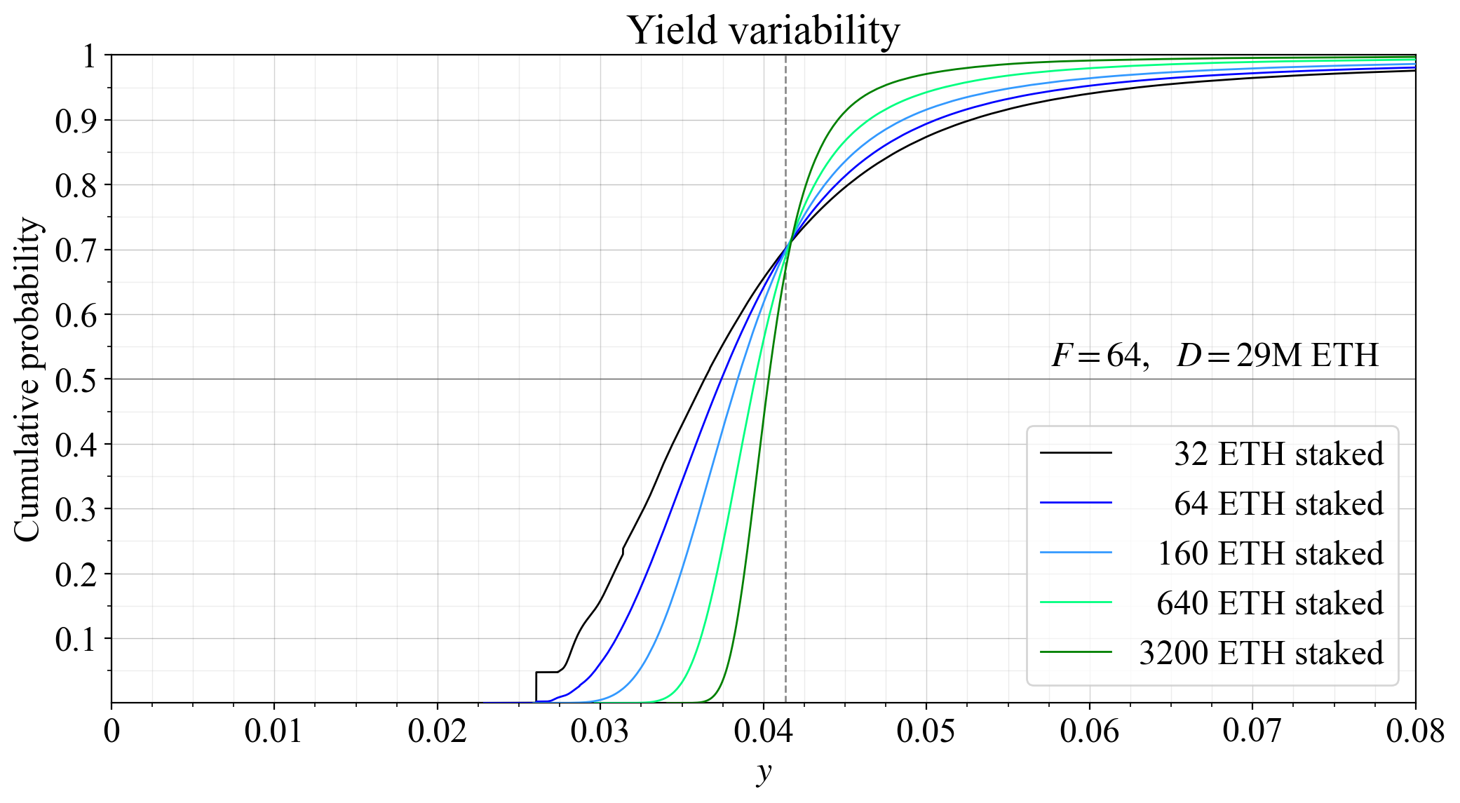
Figure 9. The influence of pooling on variability in staking yield at the current deposit size of D= 29M ETH, captured using CDFs of different pool sizes.
As illustrated in Figures 5-6, the proportion of attester rewards is around 0.5 at 29M ETH staked when F=32. This retains proper consensus incentives according to the guidelines from Section 3. But it is perfectly reasonable to expect a higher quantity of stake under equilibrium at F=32 and a staking fee would then be required to achieve an equilibrium, as previously discussed. An example of the effect of such a fee is shown in Figure 10, where the yield at 29M ETH is pushed down to 1.25 %, while keeping F=32 to retain proper consensus incentives. A yield of 1.25 % is still within the green area of Figure 6, meaning that stakers have a positive expected y_i (even when y_i accounts for the fee, as in this post). However, a black vertical section of the solo staking CDF in Figure 10 indicates a negative yield over the year for solo stakers that do not get to propose a block or attest in the sync committee. This happens because the proposer gets 1/8 of all issuance rewards (and the sync-committee attester 1/32), and so non-selected stakers must still lose ETH every epoch even as y_i is slightly above zero. Trying to push the yield into the white area of Figure 6 pushes a larger section of solo stakers underwater over a year. The notion of solo stakers being affected the worst by a low issuance yield is something that will be explored further in the following subsections. However, that analysis will not include a fee, instead focusing on the degradation that happens even without a fee.
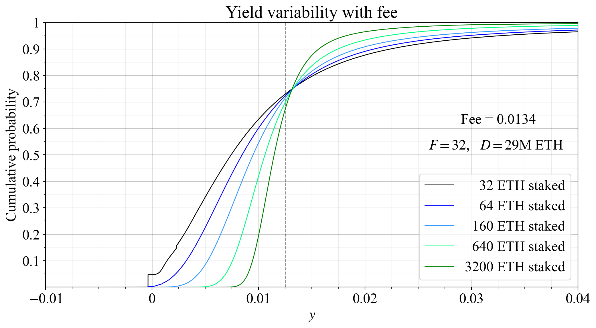
Figure 10. The influence of pooling on variability in staking yield at the current deposit size of D= 29M ETH, when applying a staking fee of 1.34 % to push down the expected staking yield to 1.25 %.
Two additional figures can be interesting, covering the situation under equilibrium with the current issuance policy and the two hypothetical supply curves. With the higher supply curve from previous plots, the equilibrium staking is around 41.9M ETH. Figure 11 shows the variability under such a deposit size, otherwise using the same conditions as previously. Average y (indicated by a grey dashed line) falls at the equilibrium.
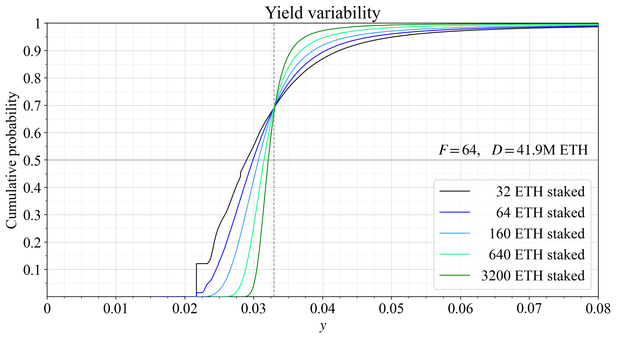
Figure 11. The influence of pooling on variability in staking yield at a hypothetical equilibrium of D= 41.9M ETH, captured using CDFs of different pool sizes.
With the lower supply curve, the equilibrium is D= 50.4M ETH, as shown in Figure 12. The vertical part of the black line, representing solo stakers with no block or sync-committee assignments, is then rather noticeable.
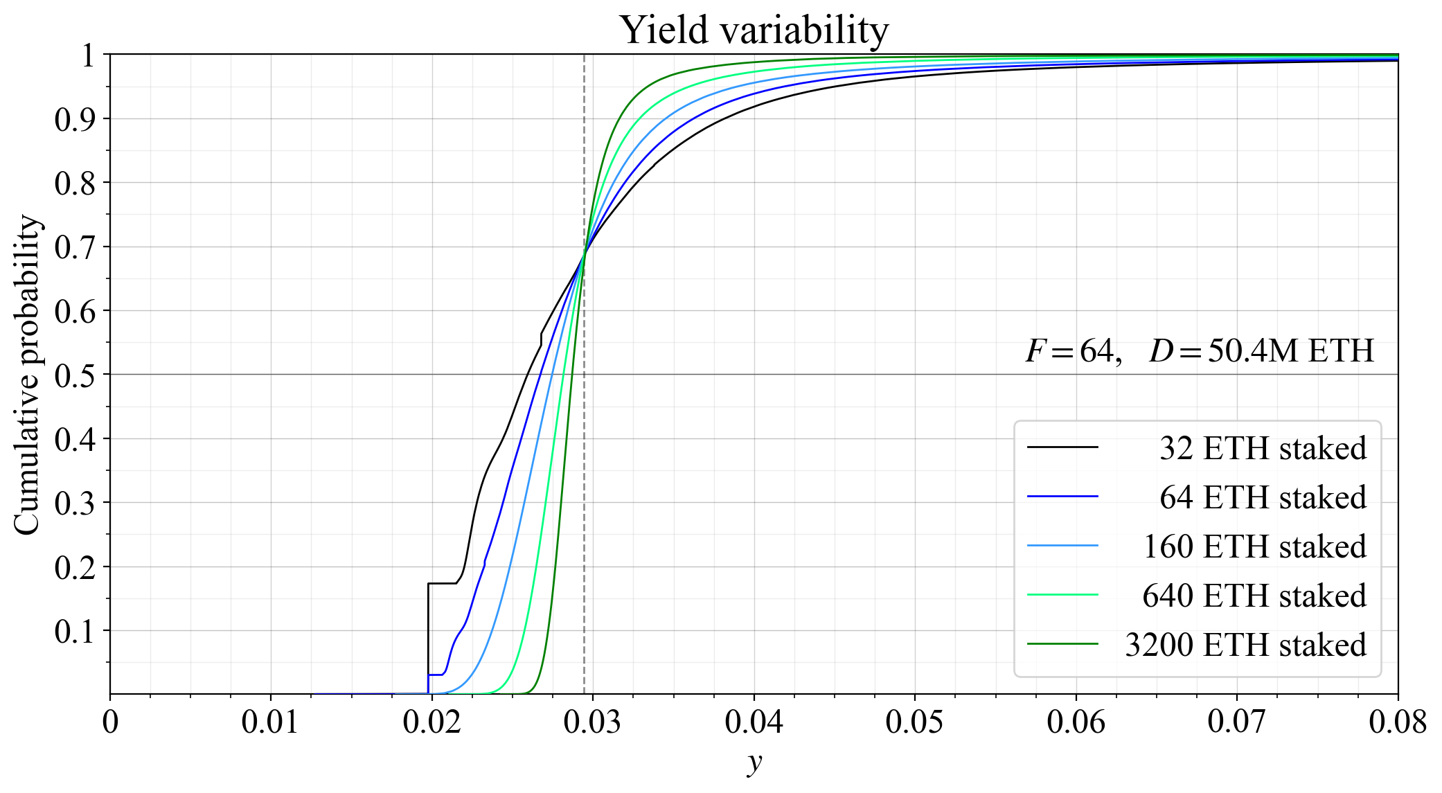
Figure 12. The influence of pooling on variability in staking yield at a hypothetical equilibrium of D= 50.4M ETH, captured using CDFs of different pool sizes.
4.3 Variability with fixed supply and varied demand
It is now time to study how variability in yield changes for solo stakers when F is changed (no fee). Figure 13 shows the equilibrium CDF under the lower supply curve (the expected yield is dashed). When F=0, only REV remains, and stakers with no block proposals receive no rewards at all.
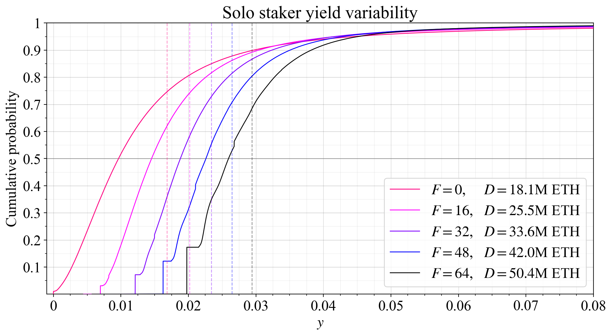
Figure 13. Changes to solo staker yield variability under equilibrium for a fixed hypothetical supply curve when F (demand) is changed.
To better illustrate the risk solo stakers take on in comparison with delegating stakers, all cumulative probability distributions were normalized by subtracting the average yield (“shift-normalized”), as shown in Figure 14. This preserves the standard deviation (SD) of each distribution. It is now easier to observe how a change to F increases variability at the medium-run equilibrium. The effect is particularly prominent at F=0, and also noticeable at F=16. From F=32 and above, the increase in variability relative to F=64 is less significant.
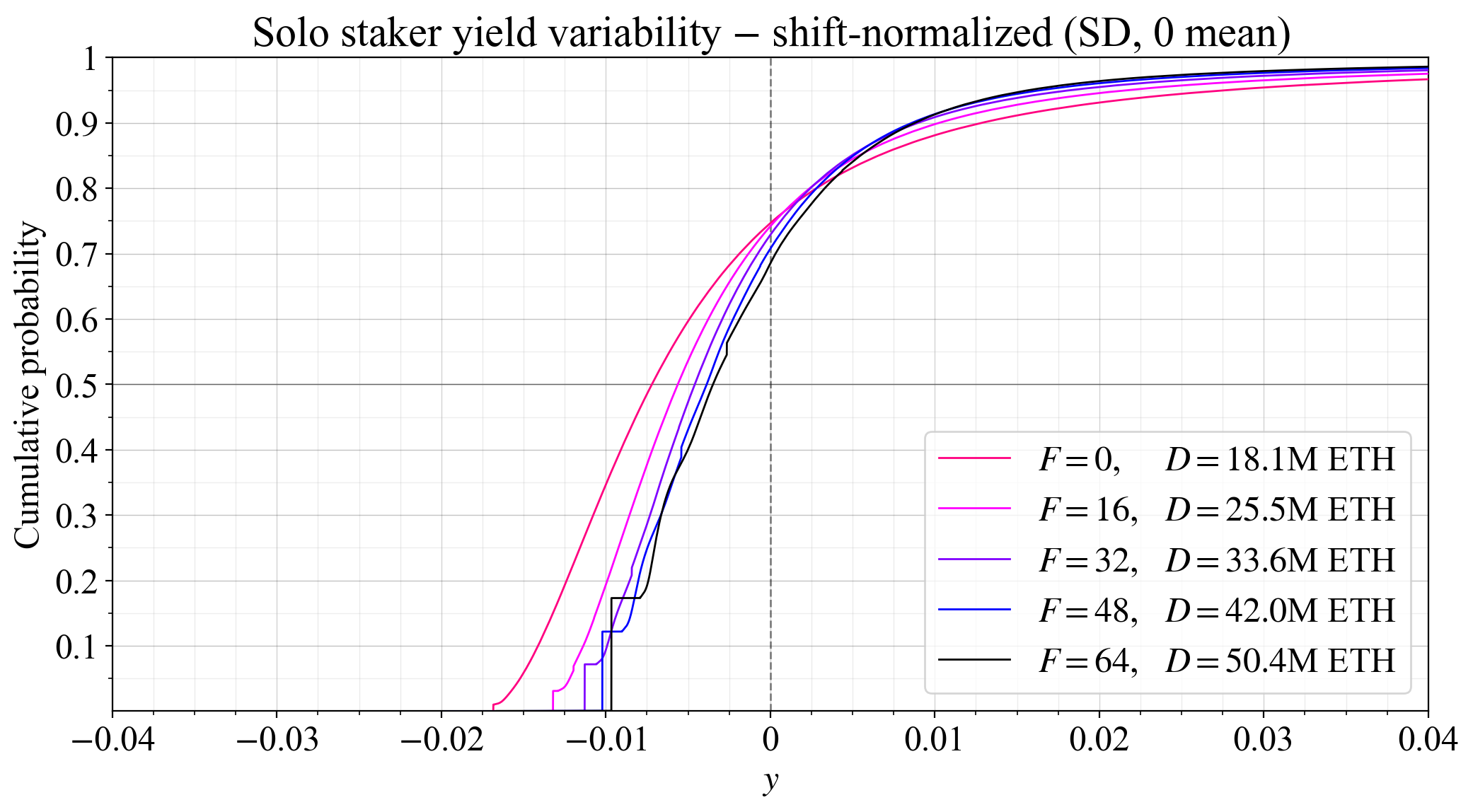
Figure 14. The CDFs from Figure 13, all shifted to have have 0 expected yield, better illustrating how variability changes.
The SD is illustrative when discussing how the shape of the distribution affects risks. But the SD (or variance) is insufficient for capturing the full impact of variability for the risk-averse staker. The higher-order moments of the distribution also matter. In particular, a positive skew is favorable. In this regard, Ethereum’s yield distribution is certainly better than its inverse, where there would be a small risk of losing everything (although the prospect of slashing indeed leads to such a risk). The worst-case scenario for honest and attentive stakers is thus an important feature.
Solo stakers may in reality be worse affected at the same SD when the expected yield is lower. As a simplified example, say that solo stakers are some fixed proportion of all stakers at any deposit size when there is no variability in rewards, and that the supply curve rises linearly. Then, if the expected yield is 2 % and can vary uniformly between 1-3 %, half of the solo stakers would need to account for the risk of receiving a yield below their reservation yield over a year. If the expected yield is 5 % but can vary between 4-6 %, the proportion affected is 1/5. Figure 15 accounts for such relative effects, instead normalizing by dividing each distribution by the ratio between its mean and the mean at F=64 (“scale-normalized”). This preserves the relative standard deviation (RSD) of the distribution, computed as SD/mean yield (mathematical notation: \sigma/\mu). From such a perspective, variability for solo stakers certainly starts to degrade already around F=32, and more so at F=16. But this is just one viewpoint on the matter, both the SD and RSD convey something important about the solo stakers’ conditions.
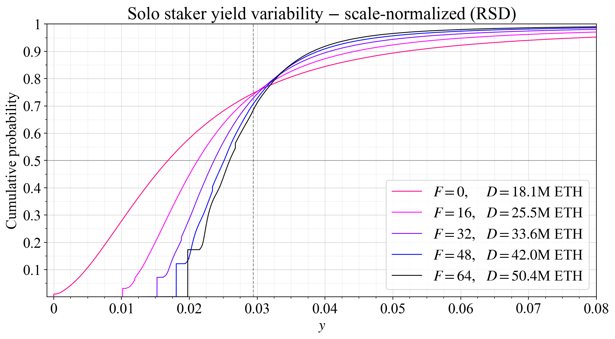
Figure 15. The CDFs from Figure 13, all “scale-normalized” (\sigma/\mu) to have the same expected yield. This preserves the relative standard deviation.
4.4 Variability with fixed demand and varied supply
Another interesting perspective is to vary D while keeping the reward curve fixed, thus computing variability across demand. This allows us to study equilibrium distributions, where each one is the result of a different supply curve. From a consensus developer’s perspective, this is a very important viewpoint and will be the focus going forward in this post. It is easier to control the shape of the demand curve (particularly after MEV burn), as opposed to the supply curve. Figure 16 shows CDFs capturing yield variability for the current reward curve at various deposit sizes. At 110M ETH staked (black line) almost half the validators will neither propose blocks nor sync-attest over the year at equilibrium (vertical line segment). The impact of special duties at such a high deposit size is indeed interesting to note. Being selected to the sync-committee gives almost as much issuance yield as attesting correctly over the full year (78 %, regardless of reward curve). But an equilibrium at D= 110M ETH requires that the marginal staker has a reservation yield below 2% at the prevailing level of REV, which seems rather unlikely for the near future.
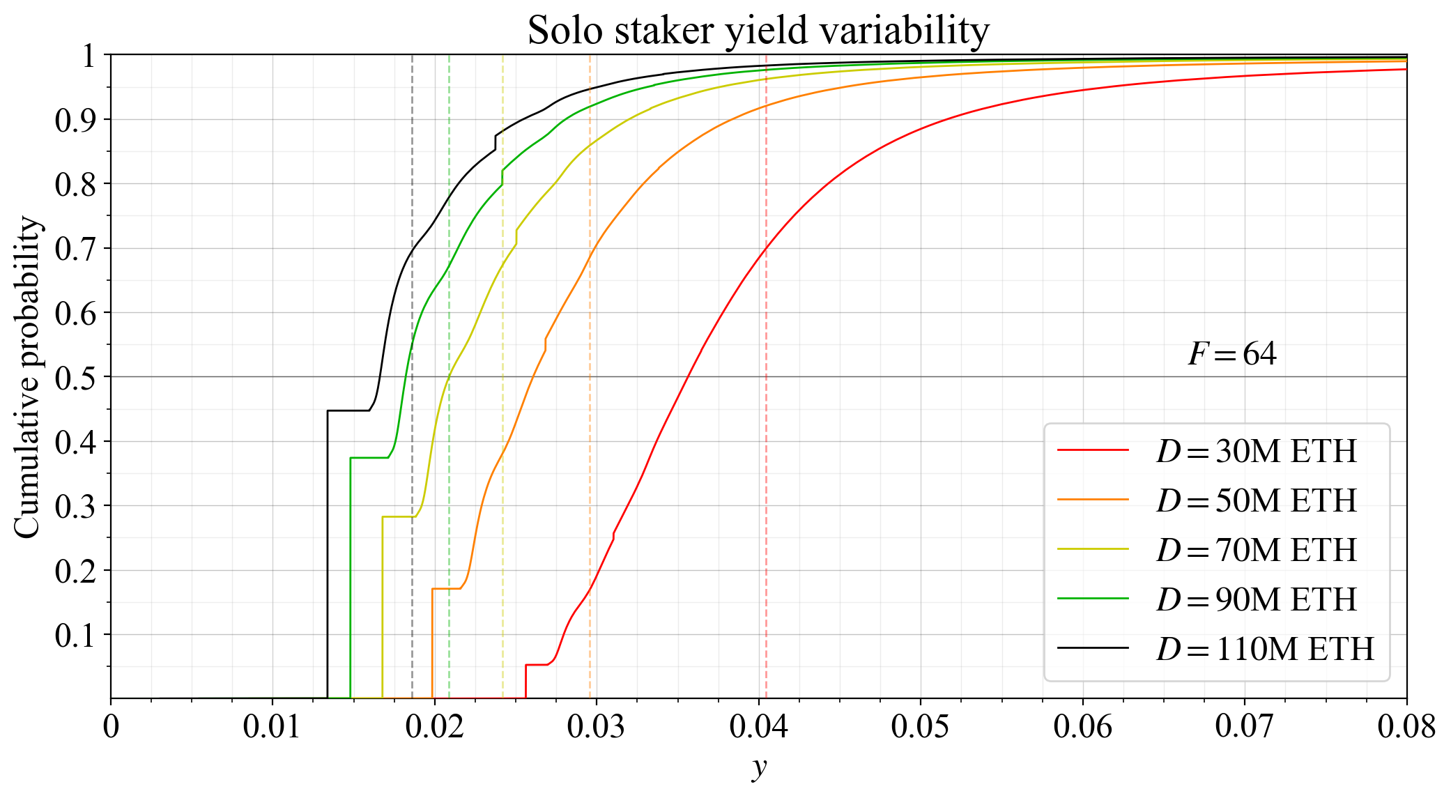
Figure 16. Solo staker yield variability at various deposit sizes under the current issuance policy.
Still, as implied by the shift-normalized distributions in Figure 17, the SD decreases with an increase in deposit size, keeping F fixed. This happens because the higher frequency of selection for special duties at lower deposit sizes serves to differentiate validator outcomes. Also remember that the standard deviation is computed after first subtracting the mean.
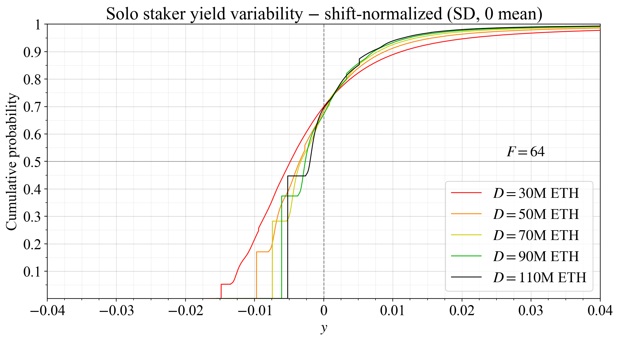
Figure 17. Solo staker yield variability at various deposit sizes under the current issuance policy, with CDFs shifted such that the expected yield is 0.
When it comes to the RSD, it is kept relatively fixed across D under the medium-run equilibrium, as indicated by the scale-normalized CDFs in Figure 18. This is opposed to the SD which is more or less fixed across F at the same D.
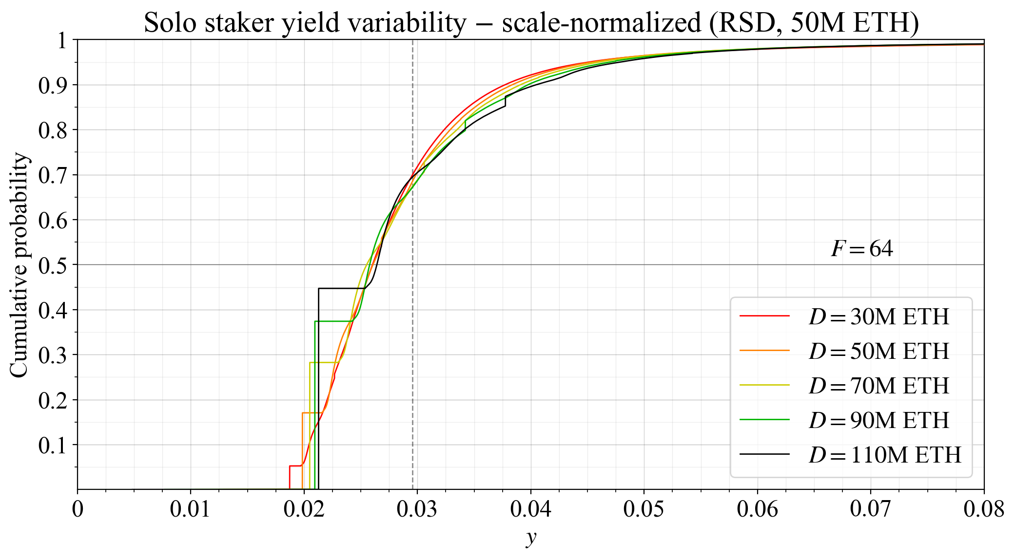
Figure 18. Solo staker yield variability at various deposit sizes under the current issuance policy as in Figure 16, but with CDFs scaled to have the same expected yield.
If F is reduced to 32, the equilibrium deposit size will fall. Ignoring this, Figure 19 shows the distributions at the same fixed D as previously. The yield at 110M ETH staked is then just above 1%, and the unlucky solo stakers with no assignment only receive around 0.7 %.
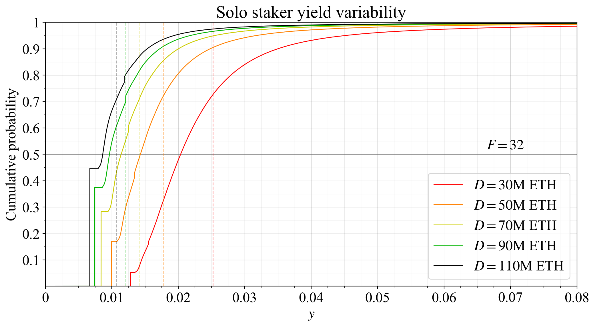
Figure 19. Solo staker yield variability at various deposit sizes when F is reduced to 32.
4.5 Two-dimensional mappings of solo-rewards variability
It can be clarifying to map the previously investigated variabilities across two dimensions, to visualize how variability changes for solo stakers across the potential equilibria. The mappings in this subsection were done by simulating solo staker’s yearly yield 10M times (sampling REV with replacement), repeated across 10^5 different deposit sizes and 32 different settings for F. The experiment was then repeated 10 times, and the measurements combined by taking the average variances. This setup was used for handling memory load since the final matrix is computed from 320 trillion simulated solo staking outcomes. Smoothing was applied across variance and mean, using a Hann window of width 1101 (across D) and height 5 (across F). The matrix was initially computed across a wider range than plotted to allow for such smoothing without artifacts. Finally, the matrix was upsampled across F.
Figure 20 shows how the SD varies across D (all the way up to 120M ETH) and F. A lower SD is better. The base reward factor has but a minuscule effect on the SD at any specific deposit size, because issuance level shifts the yield rather equally for everyone.
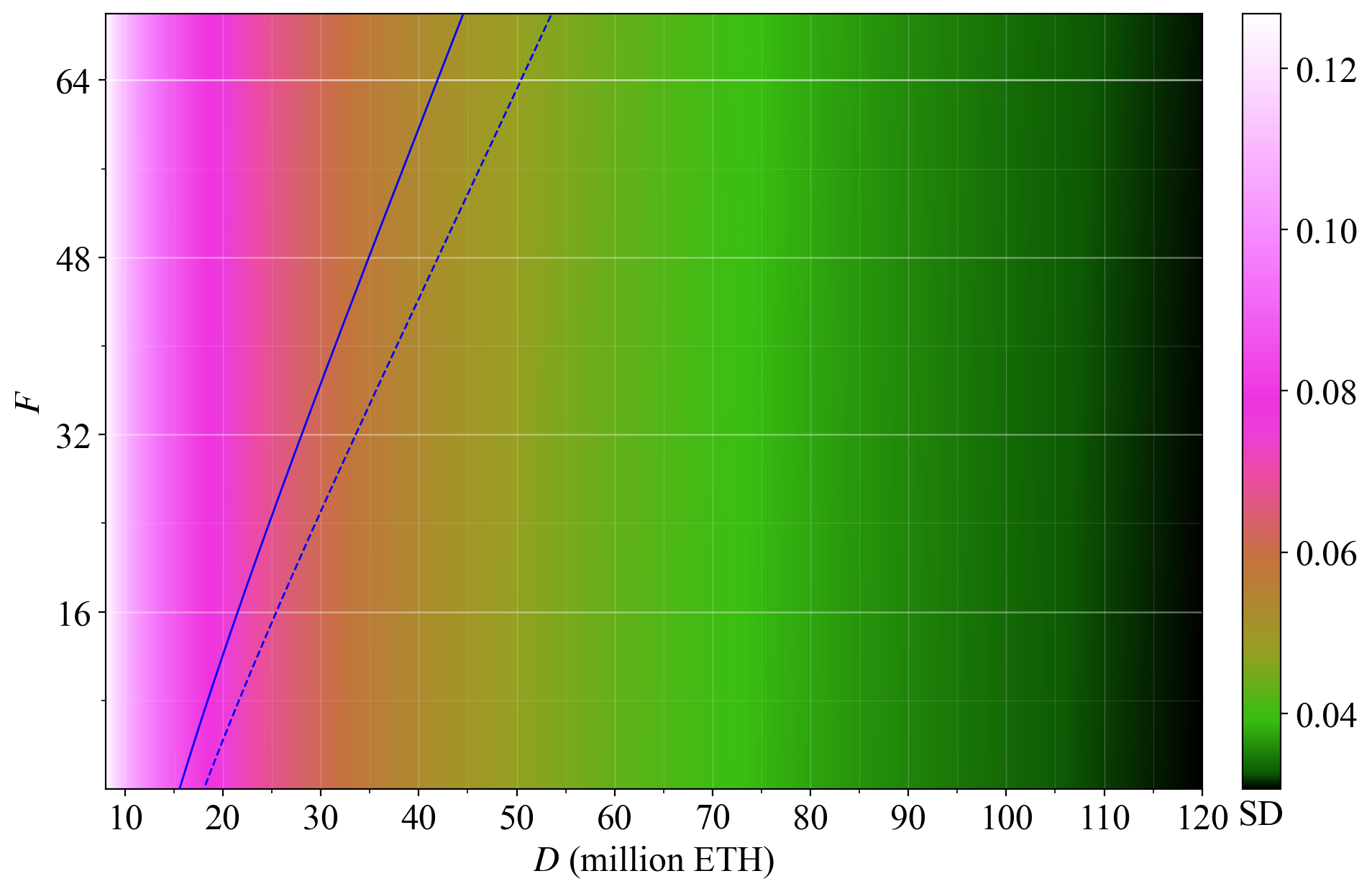
Figure 20. Standard variation in yield over a year of solo staking, plotted across F and D.
The same outcome can be observed with staking yield on the y-axis in Figure 21. To produce this graphical representation, the simulated outcome from the previous plot was simply interpolated onto the new axes. One supply curve is dashed for easier connection to the next plot.
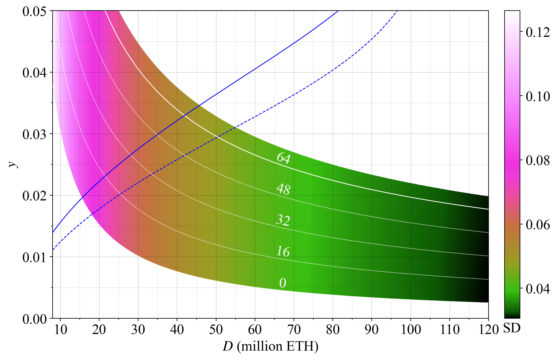
Figure 21. Standard variation in yield over a year of solo staking, plotted across y and D.
Since the quantity of stake supplied increases with a higher yield, the reality is that a higher F will produce a lower standard deviation in rewards under equilibrium. Figure 22 captures the equilibrium SD across F for the two modeled supply curves (equilibria for the lower are dashed). Thus under these assumptions, lowering F will indeed increase the equilibrium variability for solo staker while MEV burn is not in place. But the increase at 48 or even 32 is rather modest.
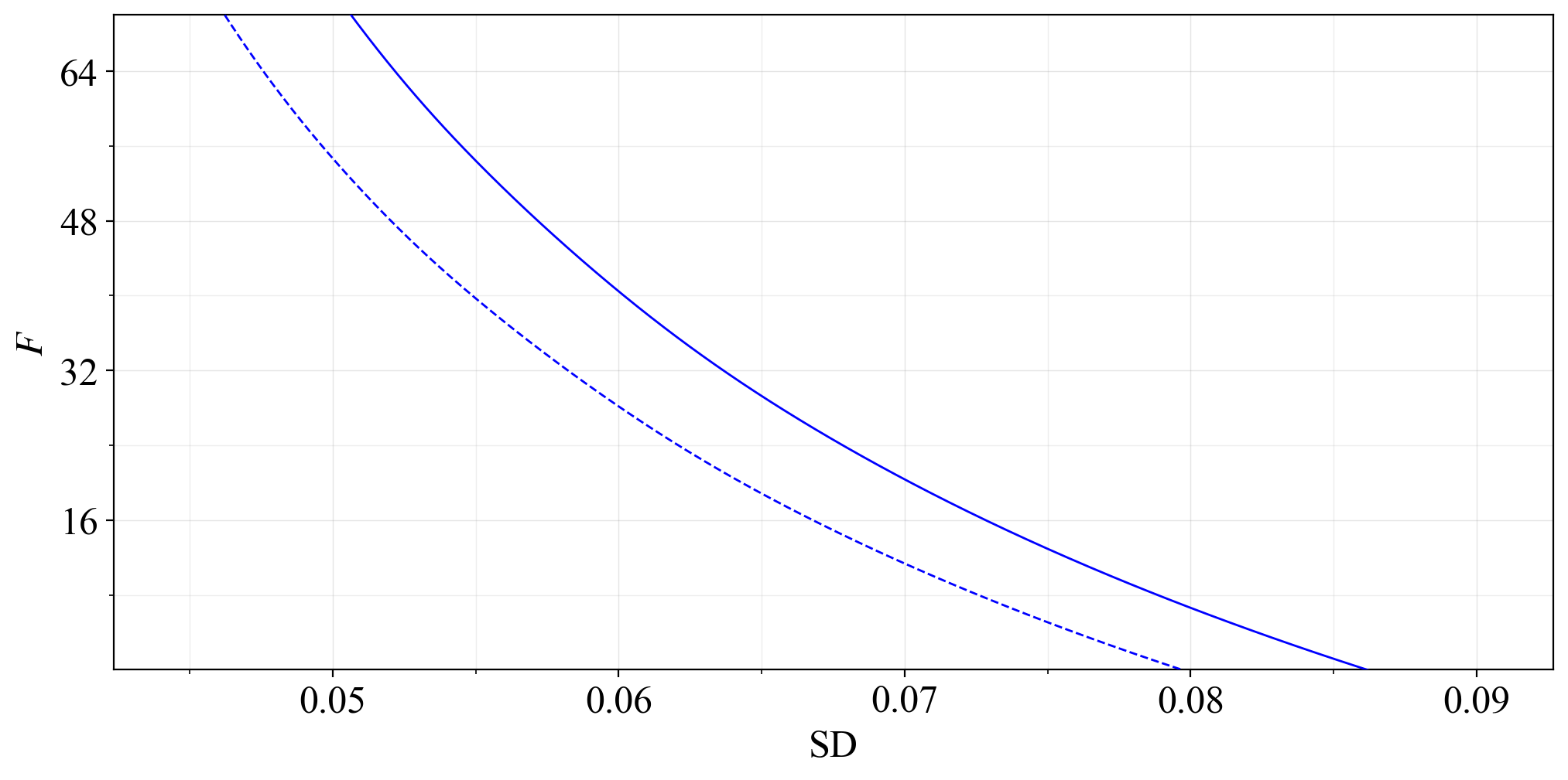
Figure 22. The equilibrium standard deviation in yield over a year of solo staking, which changes with a change to F.
Recall that another interesting perspective is the relative standard deviation (RSD), which captures the notion that a high standard deviation can be worse at a lower yield than at a higher yield. The RSD is depicted across F and D (lower is better) in Figure 23.
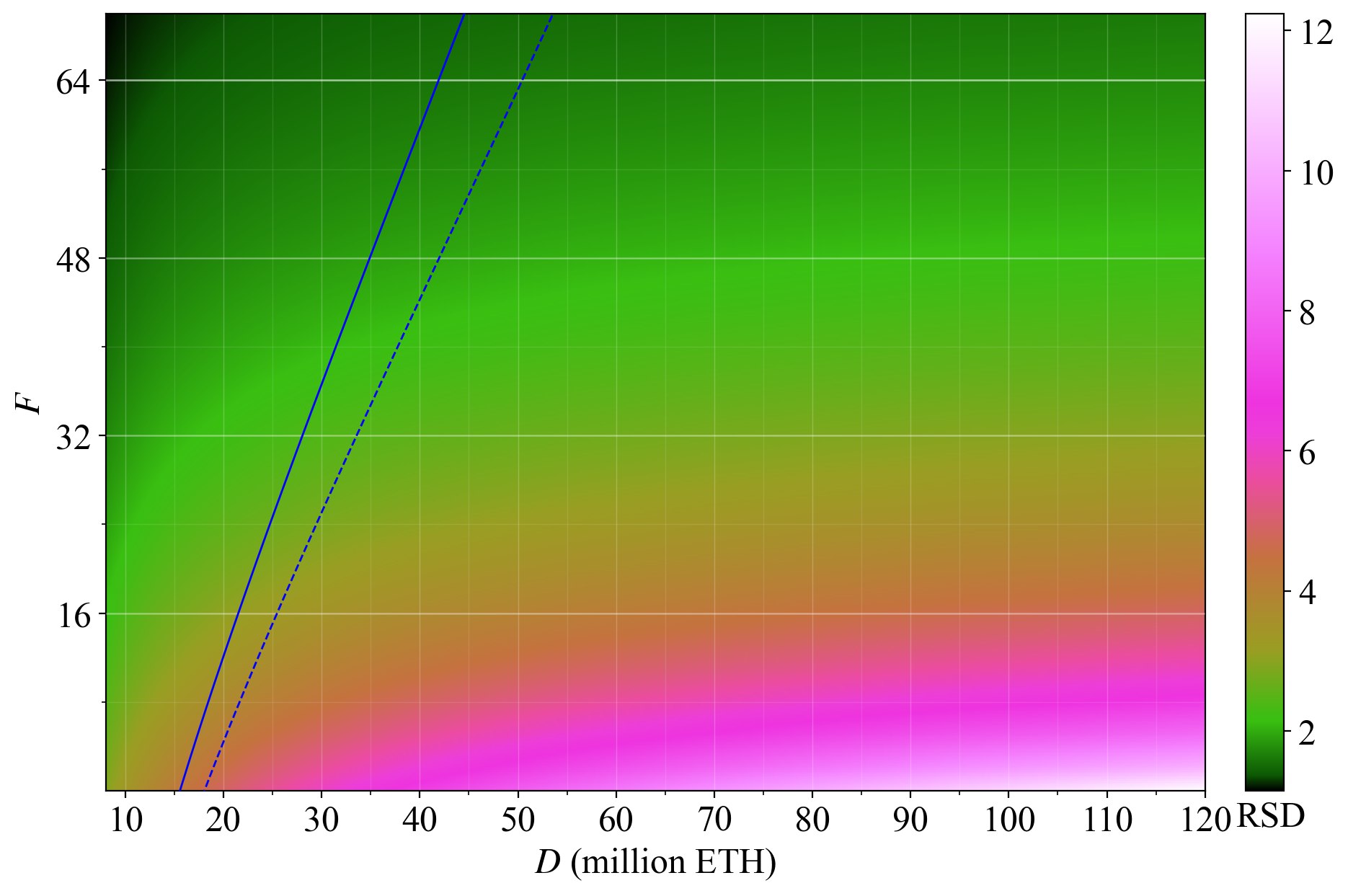
Figure 23. Relative standard variation in yield over a year of solo staking across F and D.
Figure 24 instead captures the RSD across y and D. When going by the RSD, a higher F is clearly preferable, because it serves to push up yield in general, thus facilitating a higher equilibrium yield and lower RSD.
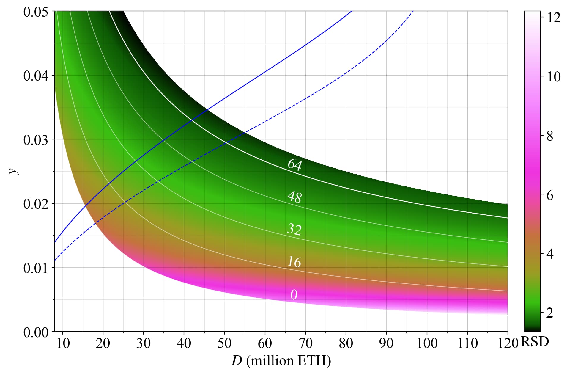
Figure 24. Relative standard variation in yield over a year of solo staking, plotted across y and D.
Arguably, the SD puts too much emphasis on variabilty and the RSD puts too much emphasis on the mean. Therefore, some measure in between these two seems appropriate for further modeling. Define the SSD as the standard deviation divided by the square root of the mean (\sigma/\sqrt{\mu}). Lower is still better. The post will use this in-between measure as a guideline for mapping relative degradation for solo stakers across various reward curves. Figures 25-26 plot the SSD. Under the combined measure, if F is kept fixed, a staking equilibrium at a higher D gives a lower SSD. To make the issuance policy more “neutral” the reward curve can be designed to produce the same SSD under any supply curve.
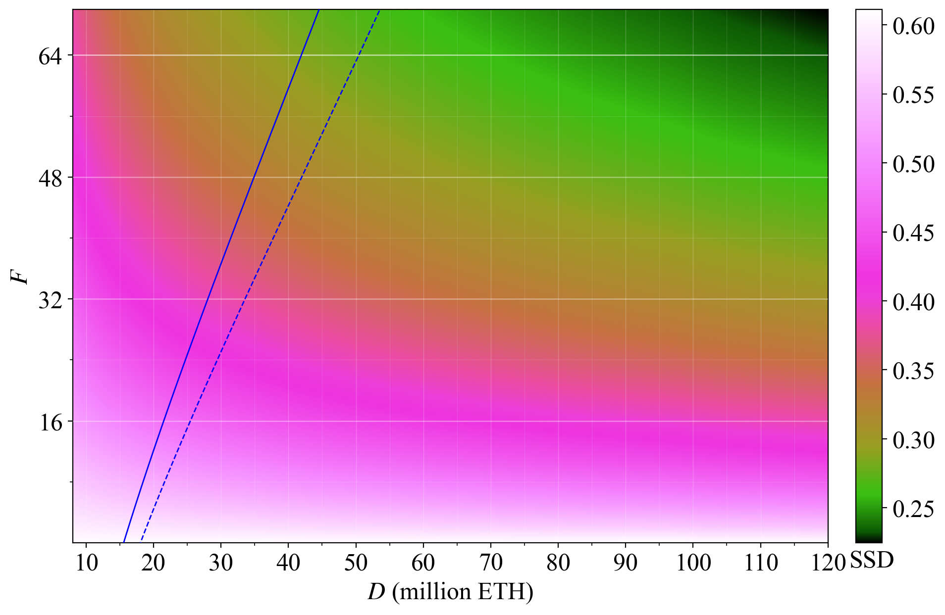
Figure 25. The SSD (\sigma/\sqrt{\mu}), capturing variability in yield over a year of solo staking across F and D (lower is better).
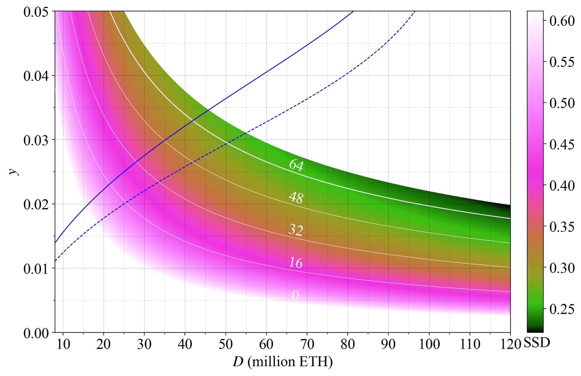
Figure 26. The SSD (\sigma/\sqrt{\mu}), capturing variability in yield over a year of solo staking across y and D.
5. Towards a utility-maximizing reward curve
5.1 A neutral reward curve
How then can a more “neutral” issuance policy, specifically a more neutral reward curve be constructed? Figure 27 plots the SSD across the reward curves with F=32 and F=64. In orange is a more neutral reward curve, preserving a set SSD at any equilibrium.
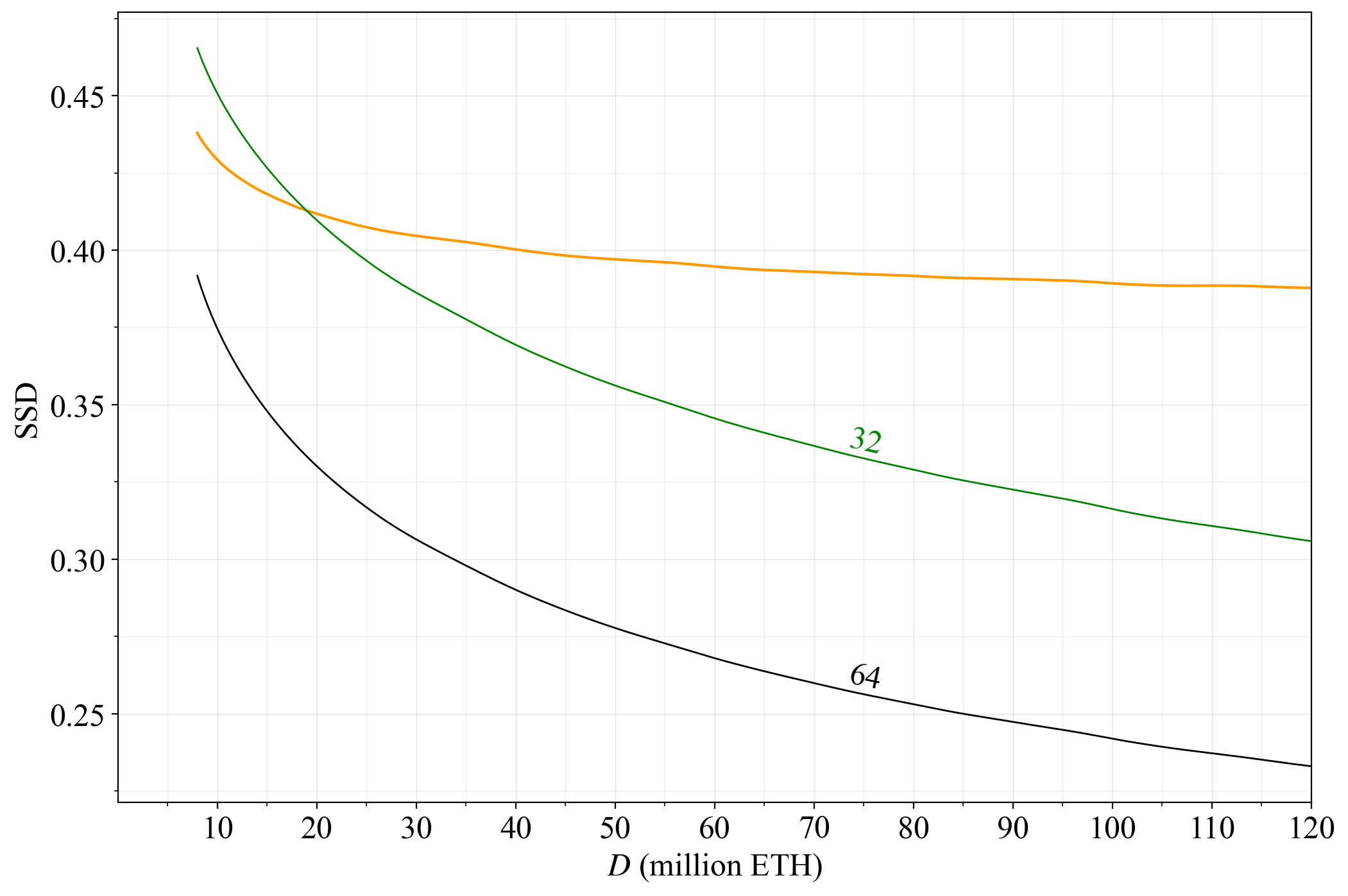
Figure 27. Variation in SSD across D for the current reward curve (black), the current reward curve but with F=32 (dark green), and a reward curve that is more “neutral” with regard to the SSD (orange).
This reward curve is also neutral across D concerning the proportion or rewards awarded to attesters, as shown in Figure 28 in the familiar plot against the attester proportion with y and D on the axes. It ensures that attestations will bring in around half of the yield at any deposit size.

Figure 28. The proportion of staking yield derived from accurately performing attester duties (as opposed to proposer duties), with y on the y-axis and D on the x-axis (see also Figure 6). The neutral reward curve in orange retains y_a/y=0.5 across almost the full range.
The equation for the reward curve is
with F=10^2 and k=2^{-11}. The difference to the current reward curve y_i=\frac{cF}{\sqrt{D}} is thus the addition of kD in the denominator and a change to F. Yearly issuance Y_i is y_i distributed across D. The equation for issuance thus becomes
This makes it clear that the reward curve is in essence a log-logistic CDF, providing an issuance level asymptotically approaching cF/k, as shown in Figure 29 that plots the yearly distributed rewards Y.
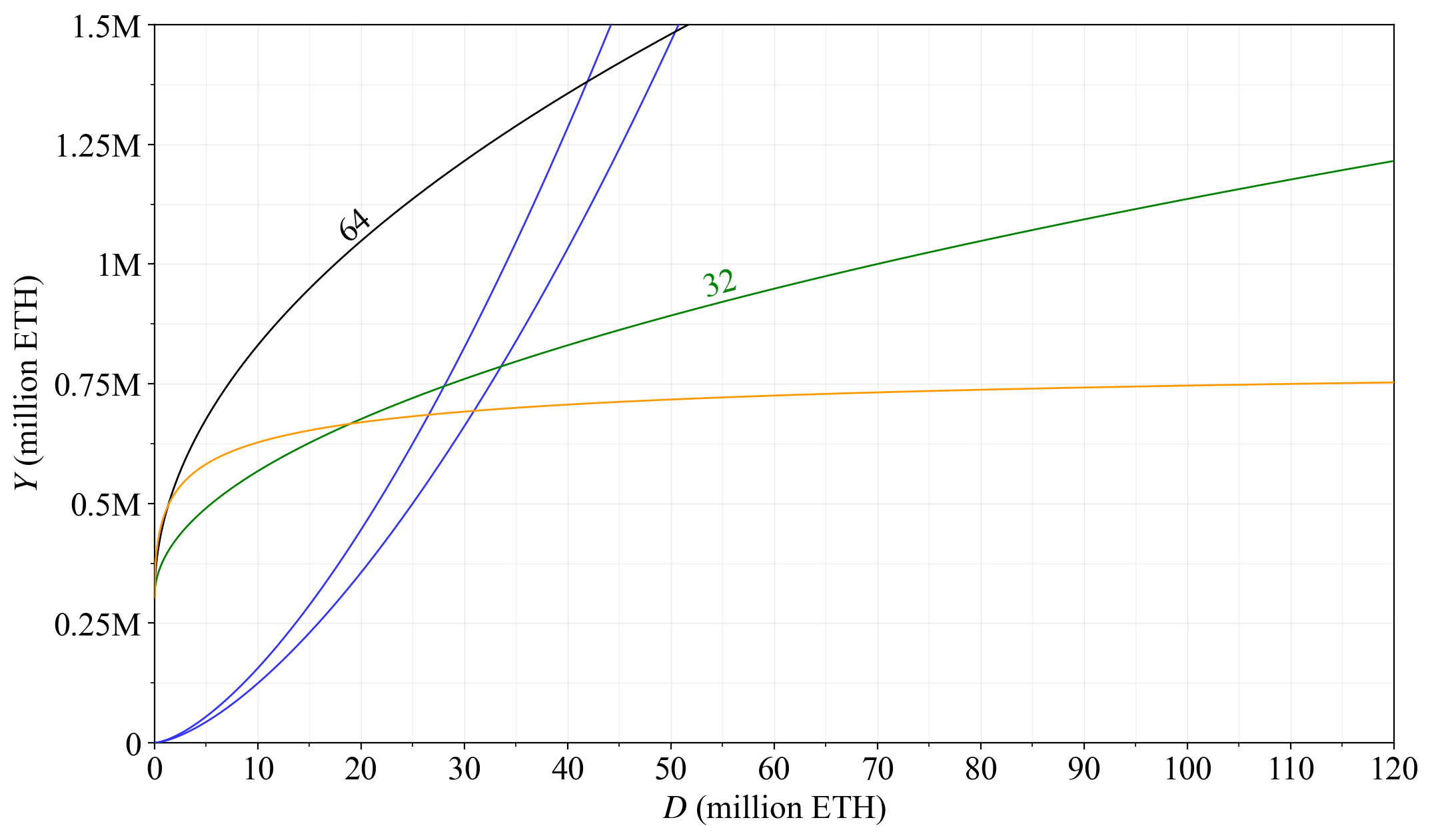
Figure 29. Yearly distributed rewards Y to stakers, with a reward curve that asymptotically approaches a fixed issuance level in orange.
In the associated thread, a functionally very similar log-logistic CDF was presented for the neutral reward curve: Y_i = \frac{2^{19}\sqrt{D}}{2^{13}+\sqrt{D}} (i.e., Y_i = \frac{2^{6}}{D^{-0.5}+2^{-13}}). In this post, all new reward curves are instead presented in the same format as the current reward curve. The purpose is to introduce as little friction as possible to the mental models around what is changed when it comes to the reward curve, and how the different presented alternatives (including the current) relate to each other. This also minimizes the required changes to the Ethereum proof of stake consensus specification (“spec”). The variable c emerges as rewards are distributed across the year. If not included, another variable must be introduced in the spec to compensate. Given the fixed constants of the spec, the relevant “base reward per increment” r_b will be r_b=\frac{\sqrt{10^9}F}{\sqrt{D}+x}, where x=kD in the first example (this equation does not account for integer arithmetics and the actual constants and operations to be applied). Various alternative examples will now be shown that alter x and sometimes F.
5.2 Exploration of alternative reward curves
The orange curve achieves some form of neutrality in terms of variability and consensus balance. It implies that Ethereum should sacrifice the same level of utility degradation in these features whatever the deposit size is. But such neutrality may not actually be desirable. Some consensus imbalance or reward variability could be acceptable to temper the deposit size if it rises very high, since a high deposit size brings utility degradation in and by itself. Furthermore, providing some safety margin at a moderate deposit size may be preferable. Table 1 explores alternative reward curves, providing a few examples using the same format as previously specified. The reward curves have been divided into various types that describe the exponentiation of D in the added term x of the denominator.
| Equation for y_i | Added variable | Color | Type |
|---|---|---|---|
| \frac{c\times64}{\sqrt{D}} | Black | R | |
| \frac{c\times32}{\sqrt{D}} | Dark green | R | |
| \frac{c\times64}{\sqrt{D}+kD} | k=0.00015 | Orange (dashed) | R_1 |
| \frac{c\times64}{\sqrt{D}(1+kD)} | k=2^{-25} | Lime | R_{1.5} |
| \frac{c\times48}{\sqrt{D}+(kD)^2} | k=2^{-19} | Pink | R_2 |
| \frac{c\times64}{\sqrt{D}+kD+(k_2D)^2} | k=2^{-14}, k_2=2^{-19} | Dark purple | R_{12} |
| \frac{c\times64}{\sqrt{D}+kD+(k_2D)^2} | k=2^{-13}, k_2=2^{-20} | Dark purple (dashed) | R_{12} |
Table 1. Equations of issuance yield for potential reward curves. The current reward curve is specified in the first row, and various reward curves created by making small adjustments are specified in subsequent rows. The third column indicates the colors of the associated curves plotted in this section and the fourth a type classification.
The yearly distributed rewards under the prevailing level of REV for the reward curves of Table 1 are plotted in Figure 30. The reward curves of type R_1 are orange in this post and have a term in the denominator that involves D, like the first neutral example. The orange dashed curve from the table however uses a relatively lower k, so it will not approach a fixed issuance as quickly. Lime-colored curves are denoted R_{1.5}, since their equation can also be expressed as \frac{cF}{\sqrt{D}+kD\sqrt{D}}. Issuance for this curve will fall as D rises, as shown in the figure. This helps Ethereum better moderate the quantity of stake once it becomes too high. An even stronger moderation is achieved by the R_2-curves (pink), adding (kD)^2 to the denominator. Finally, curves of type R_{12} (dark purple) are more versatile. The benefit of using two variables is that k can be tuned to push down the issuance as desired around deposit sizes of around 30M ETH and k_2 for pushing down the issuance at higher deposit sizes. Two variants with different focus are illustrated in the figure.
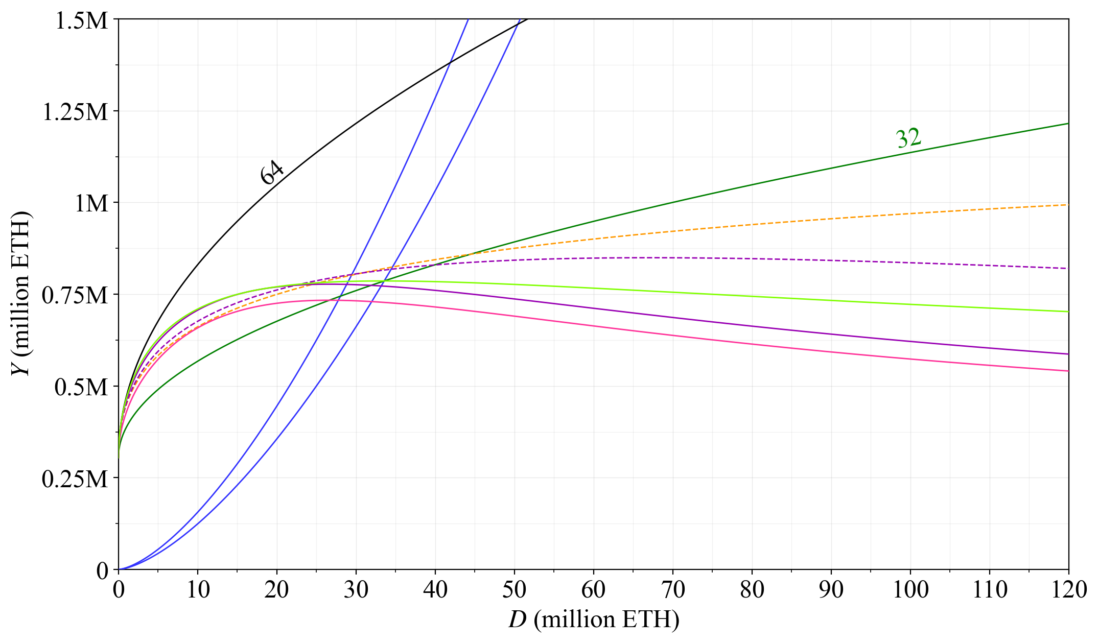
Figure 30. Yearly distributed rewards Y to stakers for the reward curves in Table 1.
Figure 31 instead shows the outcome if REV is removed, for example via MEV burn, thus plotting only yearly issuance Y_i. As illustrated, the exemplified reward curves have been designed to give a quantity of stake well above D= 14M ETH under MEV burn with the hypothetical supply curves, and would bring about an equilibrium close to the desired range.
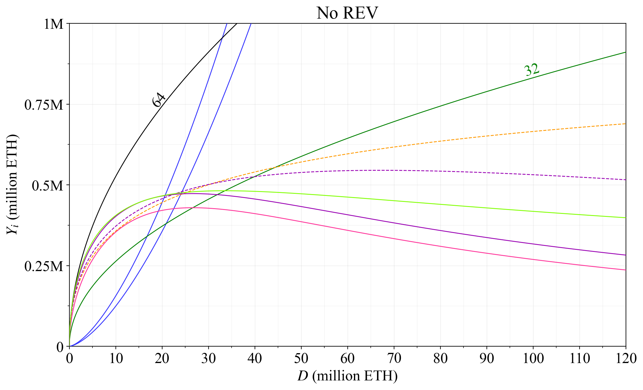
Figure 31. Yearly issuance Y_i to stakers for the reward curves in Table 1.
Figure 32 shows the staking yield y under these reward curves and prevailing level of REV. It will indeed fall quite low when D is high. Figure 33 instead plots issuance yield y_i, which of course is lower since REV is not included.
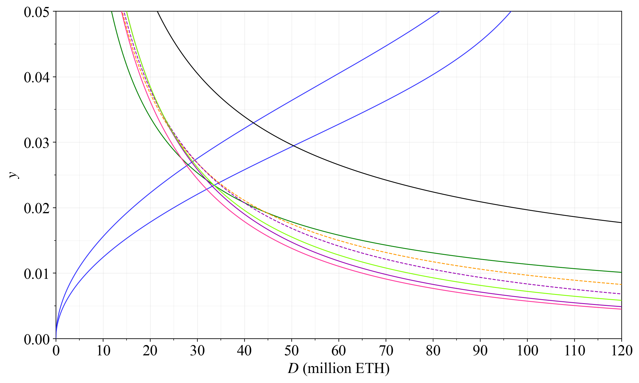
Figure 32. Staking yield y of the reward curves in Table 1.
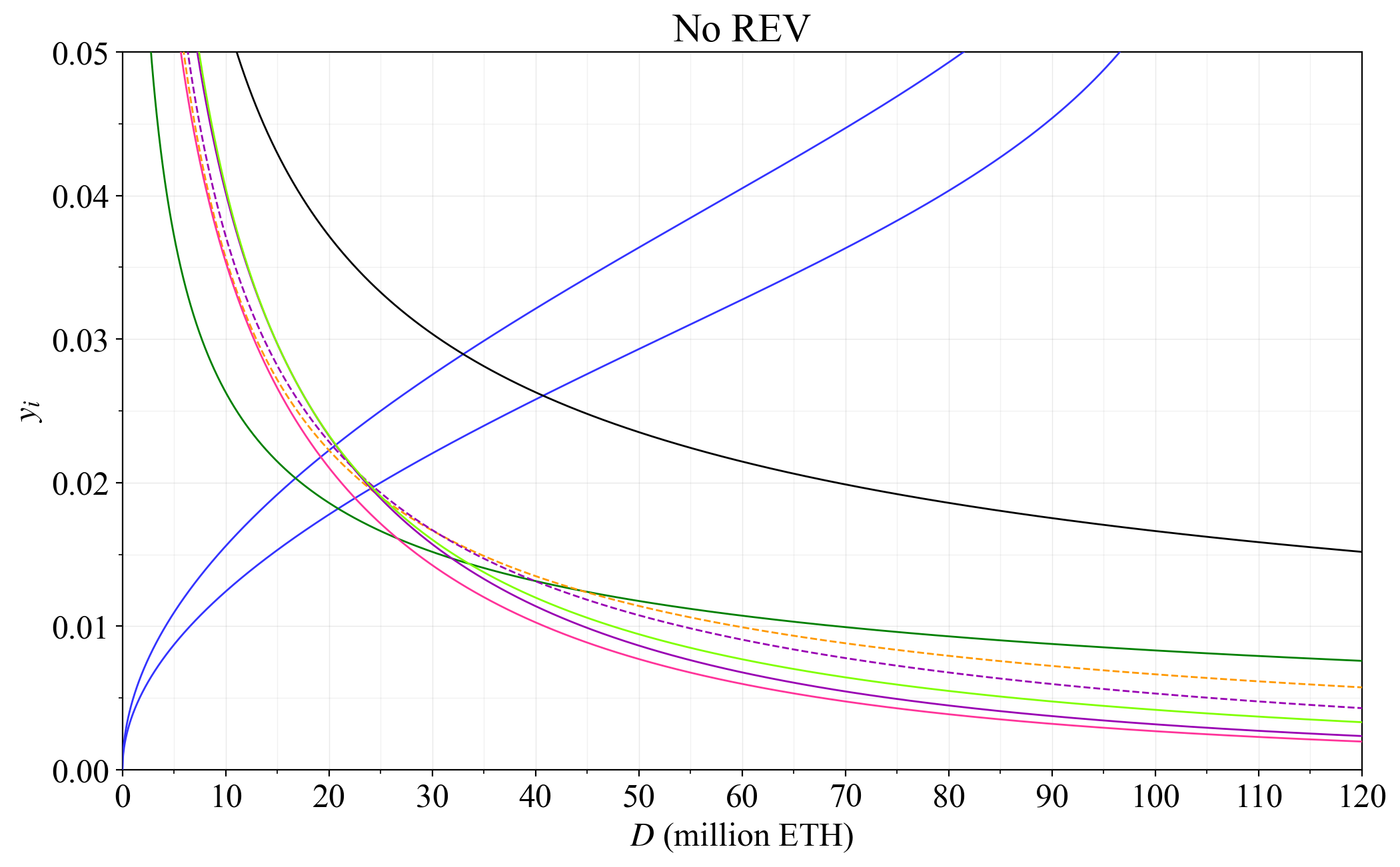
Figure 33. Issuance yield y_i of the reward curves in Table 1.
To provide a sense of how parameter settings influence the different curves, Figure 34 plots yearly issuance for each different type with alternative settings also included. Changes to parameters in curves not already specified (e.g., in Table 1) is indicated in the plot.
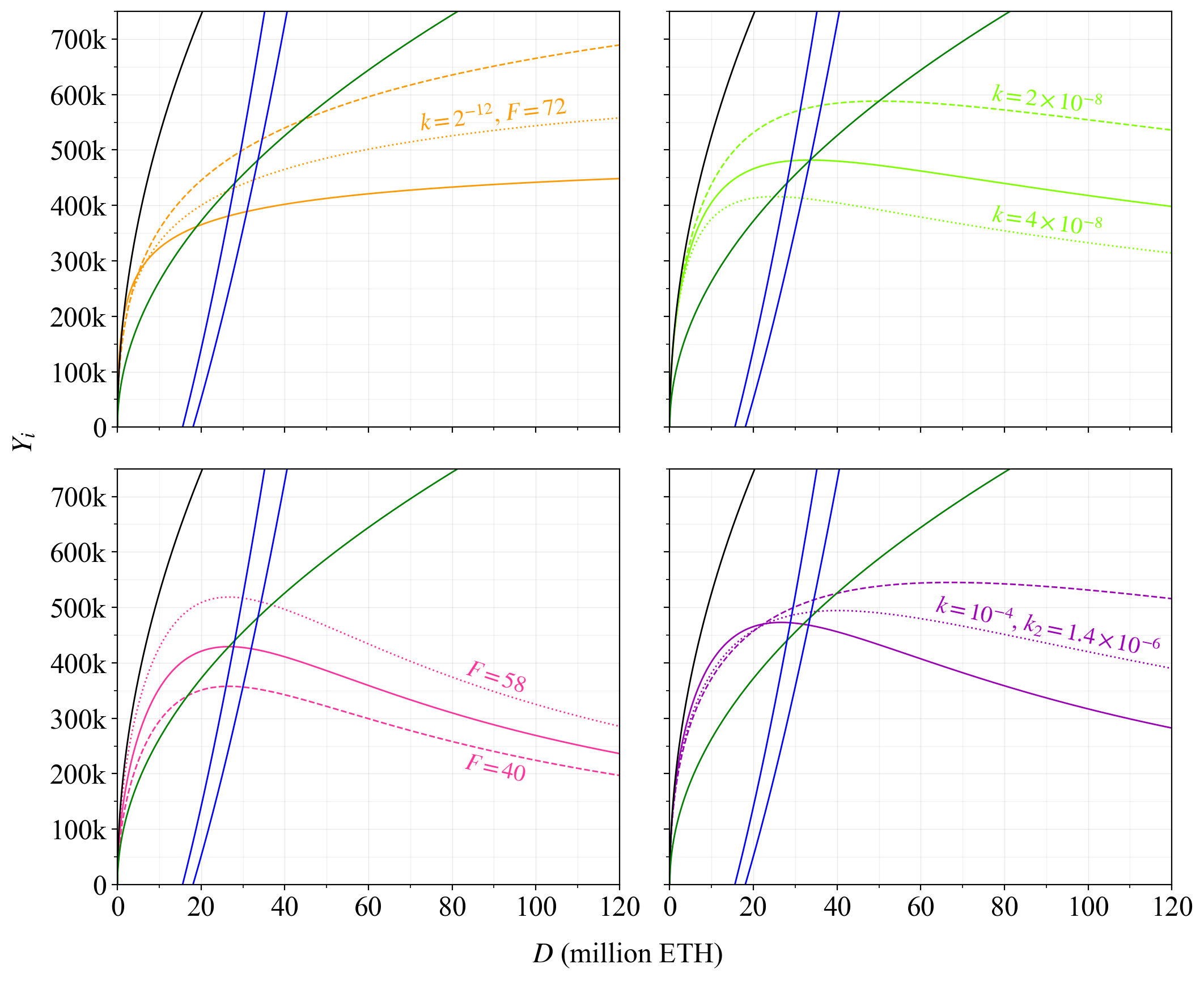
Figure 34. Yearly issuance Y_i to stakers for the reward curves in Table 1 (grouped by type), with alternative parameterizations also provided.
5.3 Analysis of the alternative reward curves
Figure 35 shows the attester’s proportion of the staking yield for the reward curves, this time having y_a/y directly on the y-axis for improved clarity. As evident, all of the analyzed reward curves will have some section with y_a/y>0.5. While the R_{1.5}-curve (lime) indeed falls with a higher D, it is still kept above 0.5 for almost the entire range. One reason why this may be reasonable is that REV is not a fixed variable. It can very well rise quite a bit, something that is out of the control of consensus developers. If the aim is to keep the proportion of the yield awarded for attestations above 0.5, then some safety margin may be reasonable.
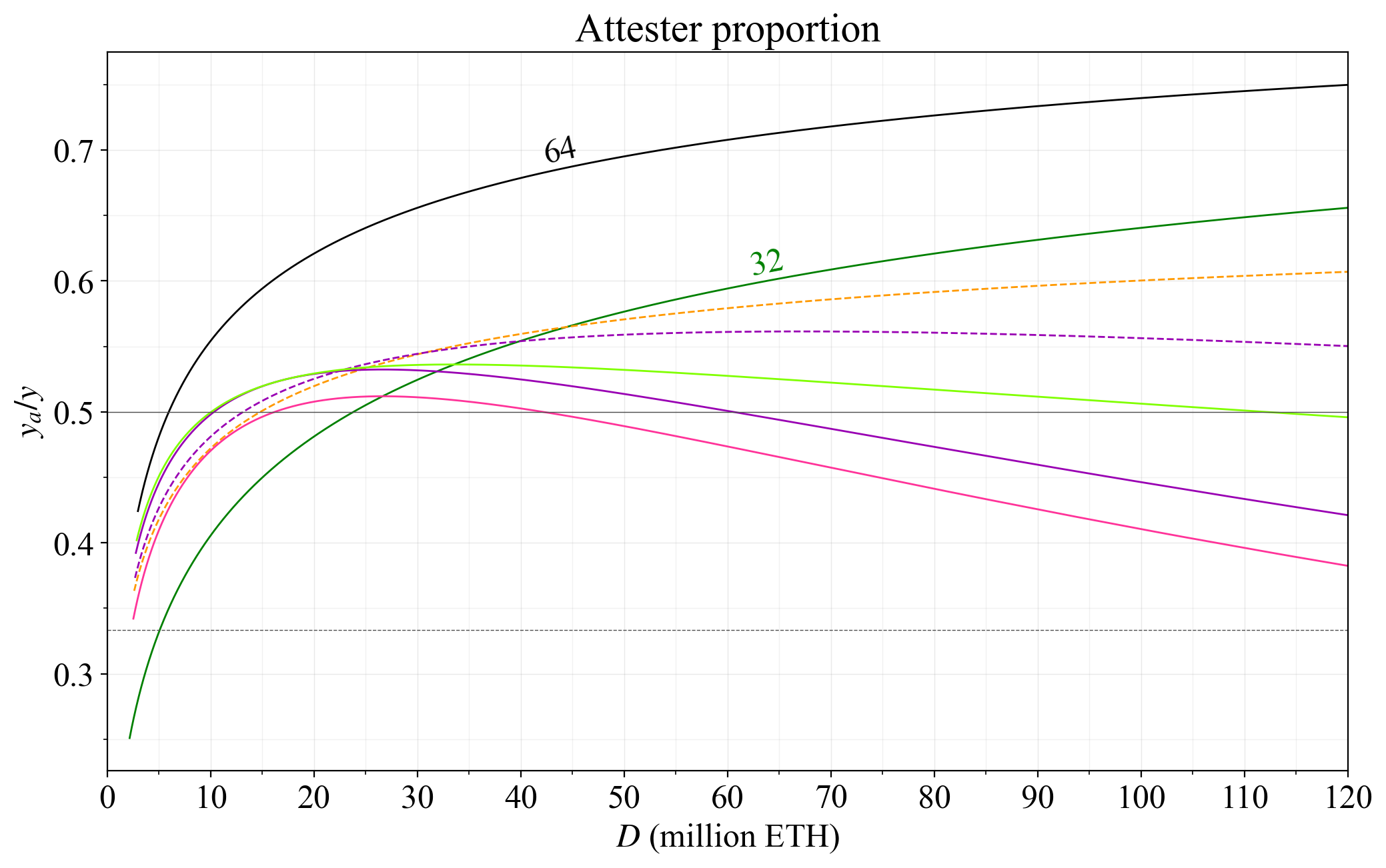
Figure 35. Proportion of the staking yield provided for attestations (y_a/y) under the current REV for the different reward curves of Table 1.
Figure 36 instead shows the situation if REV was to double. In this scenario, Ethereum will be operating under a consensus mechanism where the proposers bring in more than half of the rewards with most of the analyzed reward curves. Factoring in potential future variation in REV lends weight to using a reward curve with a somewhat higher issuance level than the most restrictive example in pink. For example, the R_{1.5} curve in lime still gives above 1/3 (dashed thin line) of the yield to attesters if the REV were to double. There is also a Bayesian aspect to these considerations. It is more likely that the equilibrium quantity of stake is higher when REV is higher, here referring to the influence of the demand curve \overline{y} on the equilibrium quantity of stake.
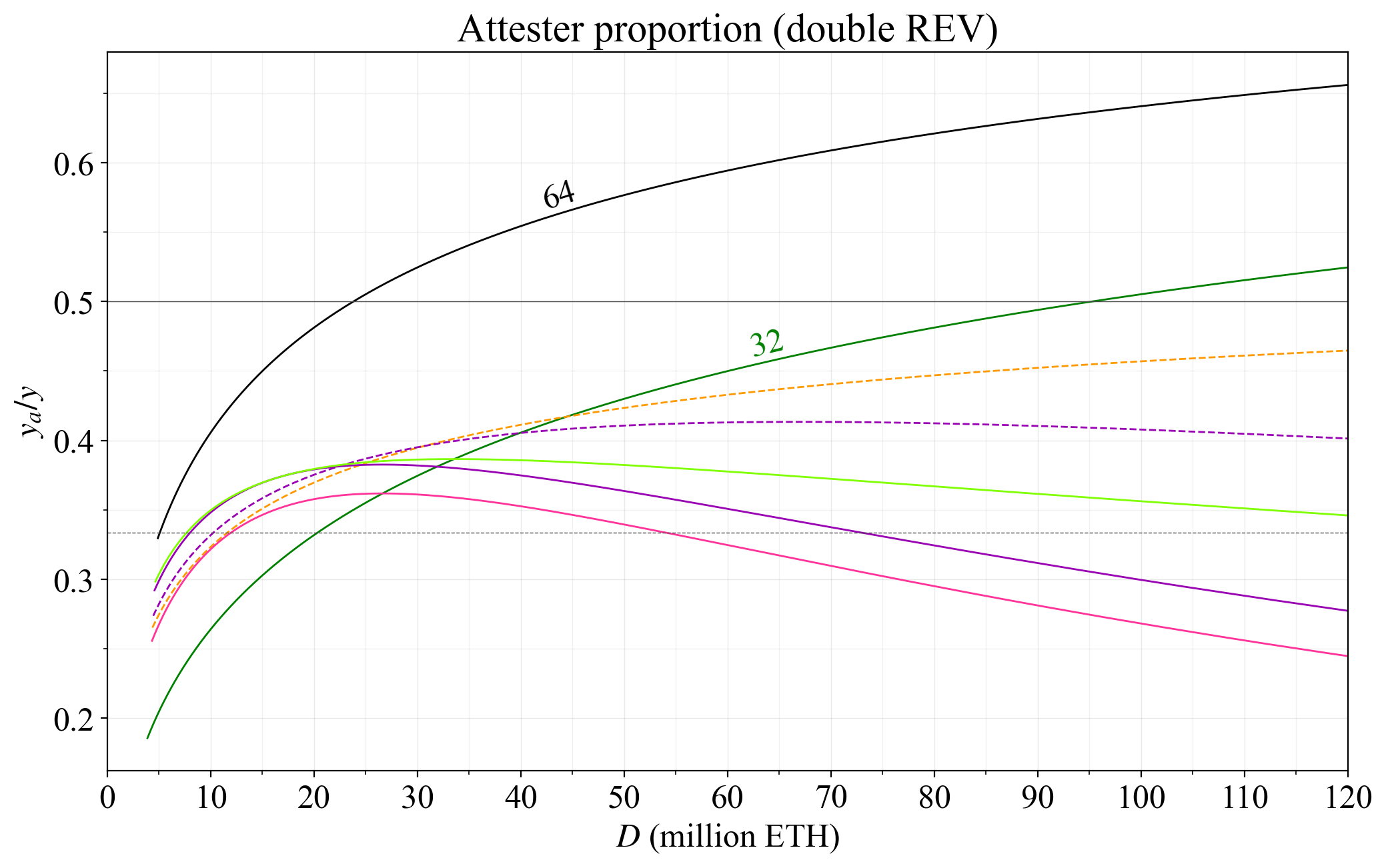
Figure 36. Proportion of the staking yield provided for attestations (y_a/y) if the REV were to double. As in Figure 35, the outcome is provided for the different reward curves of Table 1.
Figure 37 shows the SSD for the analyzed reward curves. As can be expected, the SSD rises with an increase in D for the reward curves that stipulate a falling issuance with an increase in D.
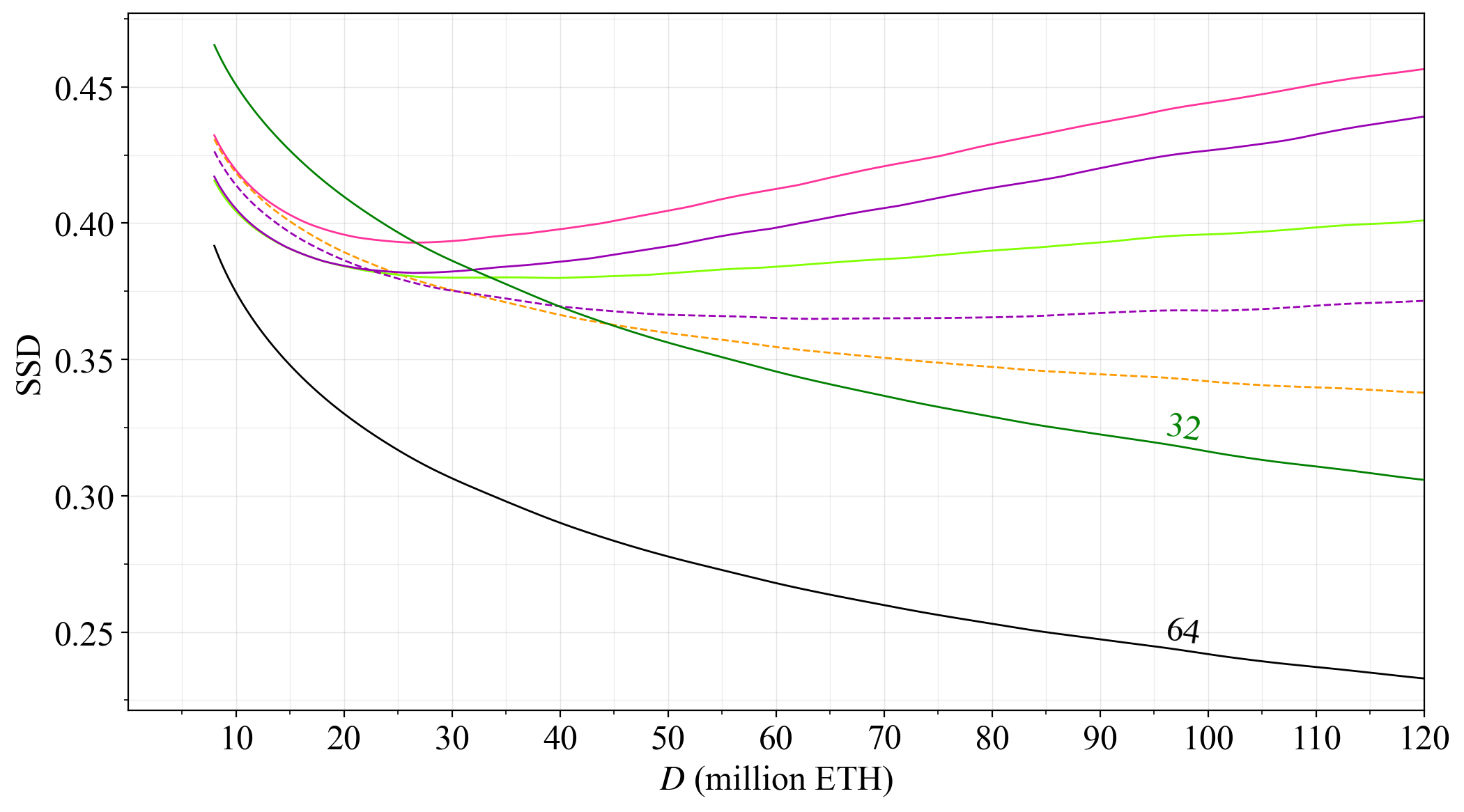
Figure 37. Variation in SSD across D for the reward curves of Table 1.
Figure 38 takes a closer look at variability for solo stakers across D under the restrictive pink reward curve. At D= 110M ETH (black line), the expected yield is around 0.5 %, and the unfortunate 45 % of stakers without special duties over the year earn just around 0.2 % in yield.
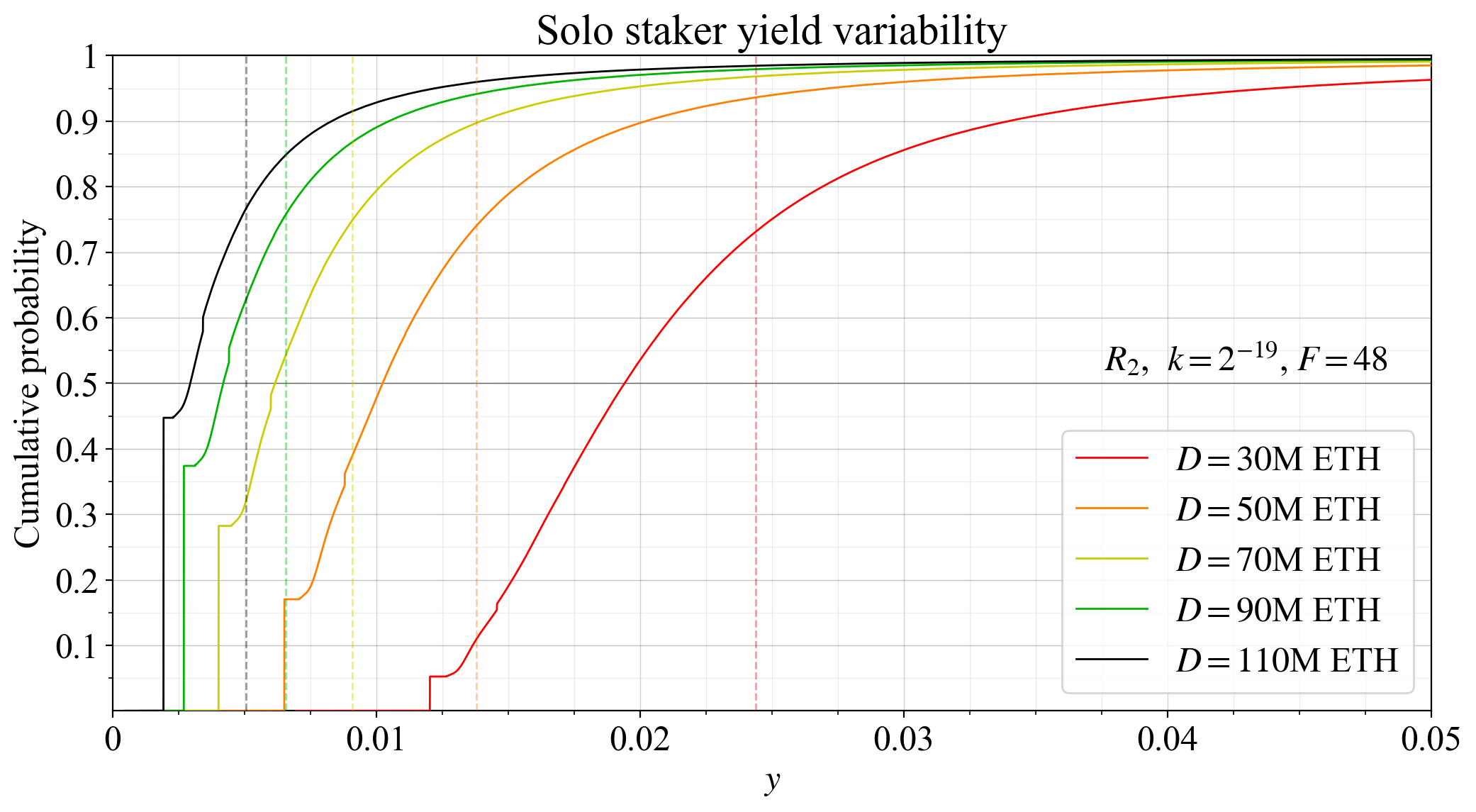
Figure 38. Solo staker yield variability at various deposit sizes under the R_2 reward curve of Table 1 (pink curve in figures).
The R_{1.5} reward curve (lime color) from previously is instead presented in Figure 39. The expected yield at D= 110M ETH is 0.65 % with solo stakers not assigned for special duties receiving 0.31 % under ideal performance. Of course, D= 110M ETH is not a likely medium-run equilibrium under either the R_2 (pink) or R_{1.5} (lime) reward curve. Indeed it cannot even be reached for several years due to the churn limit. More interesting is probably to study the red and orange CDFs in the plot, representing the variability at D= 30M ETH and D= 50M ETH respectively. The expected yield at D= 50M ETH is 1.55 %. There are fewer unlucky solo stakers in this case; around 17 % of validators are not assigned to special duties over the year, and they then receive a yield of around 0.8 % under optimal performance. Note that since the supply curve is presumably upwards sloping, the equilibrium quantity of stake is lower with the lime-colored reward curve than under the current issuance policy. With the upper hypothetical supply curve from previously, the equilibrium is slightly below D= 30M ETH and with the lower supply curve it is slightly above D= 30M ETH. The red CDF is therefore a very reasonable outcome to consider, and as evident, the unlucky validators are here much better off and further in between.
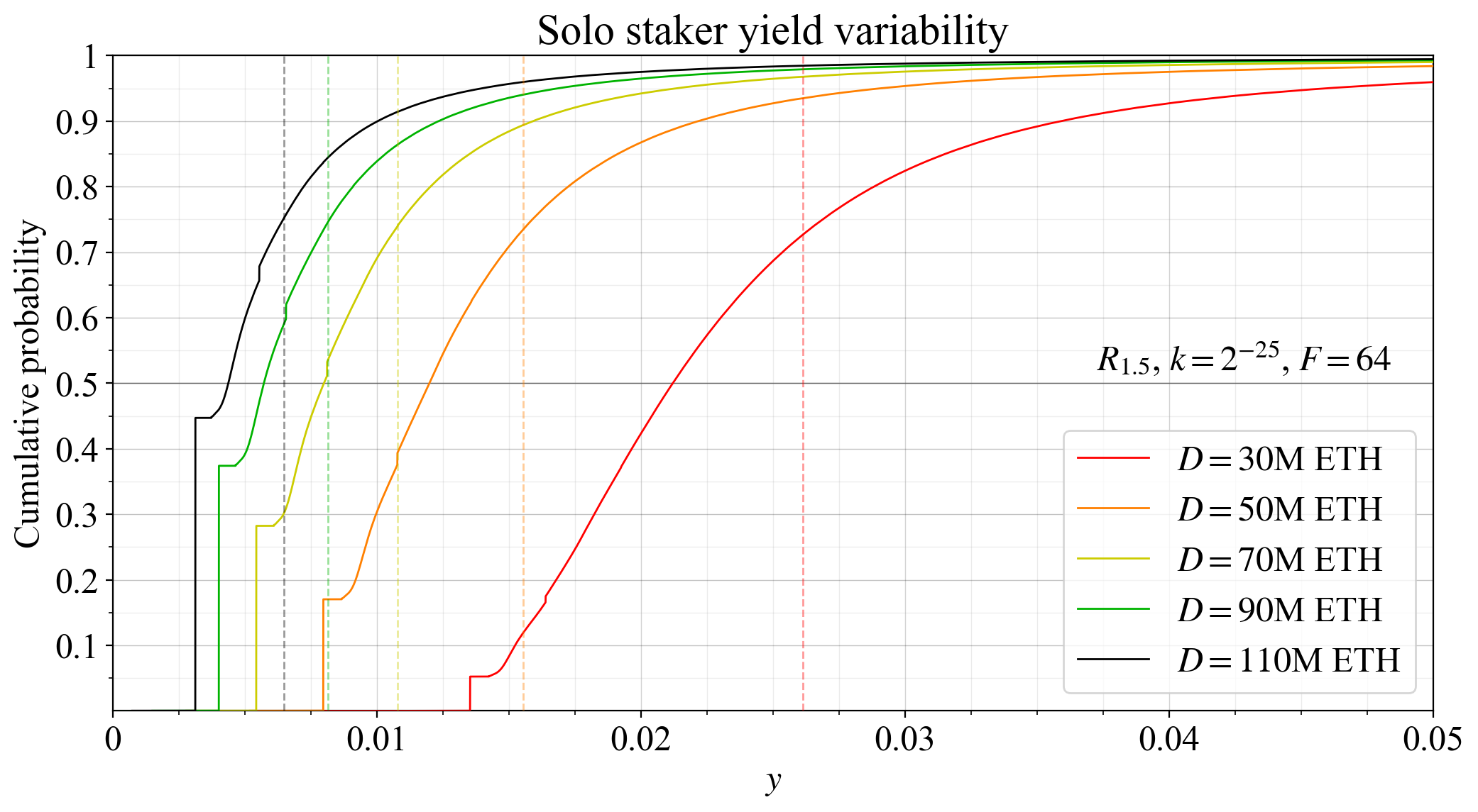
Figure 39. Solo staker yield variability at various deposit sizes under the R_{1.5} reward curve of Table 1 (lime curve in figures).
5.4 Additional properties under consideration
One aspect not covered in this post is the minimum yield under which solo staking on an efficient setup is feasible. The protocol facilitates 32 ETH solo validators and should thus ensure that y covers their minimum operational costs. Other outcomes seem pathological. Such considerations lend weight to providing some—albeit still very small—yield even at high D, so that economies of scale can never completely eliminate solo staking. These aspects will be further discussed in forthcoming analysis.
When it comes to discouragement attacks, Buterin framed his early analysis around the variable p from the equation for issuance yield of the current reward curve y_i = cFD^{-p}, with p=0.5. His paper discusses an idealized attack with a linearly rising supply curve (yield elasticity of supply equaling 1), and suggests that p>0.5 would render the attack profitable. I would first like to note that once we consider that an attacker must also de-stake under the assumption that it operates under the same supply curve, the condition actually becomes p>1. A deeper analysis will be provided in a future publication. However, these specific values for p are not hard limits. First of all, they depend on the actual supply curve and frictions. More importantly, any analysis must be weighed against the fact that an attacker will indeed put its entire stake at risk of social slashing when executing the attack.
Going deeper, we can generalize p to be the negated inverse issuance-yield elasticity of demand, hereinafter referred to as the “p_i-elasticity”. It is then easy to see following standard economics that an equivalent pointwise p_i-elasticity can be computed for any reward curve by relating the percentage change in deposit size \Delta D/D to a percentage change in issuance yield across the demand curve \Delta y_i/y_i
Figure 40 plots p_i for various reward curves analyzed in this post. I have long been in favor of a p_i-elasticity of 1 for moderating yield. The R_{1.5} curve (lime) will indeed cross p_i>1, but only if D>2^{25}, and it still remains moderate. If there is a targeting of a specific deposit size or deposit ratio, then p_i\rightarrow\infty at longer time scales (red dashed line). Such practices make a system particularly fragile to discouragement attacks. There are ways to try to resolve this beyond the scope of this post. When including REV, the negated inverse elasticity will be pushed somewhat towards 1. I will provide a deeper analysis of discouragement attacks in two forthcoming papers.
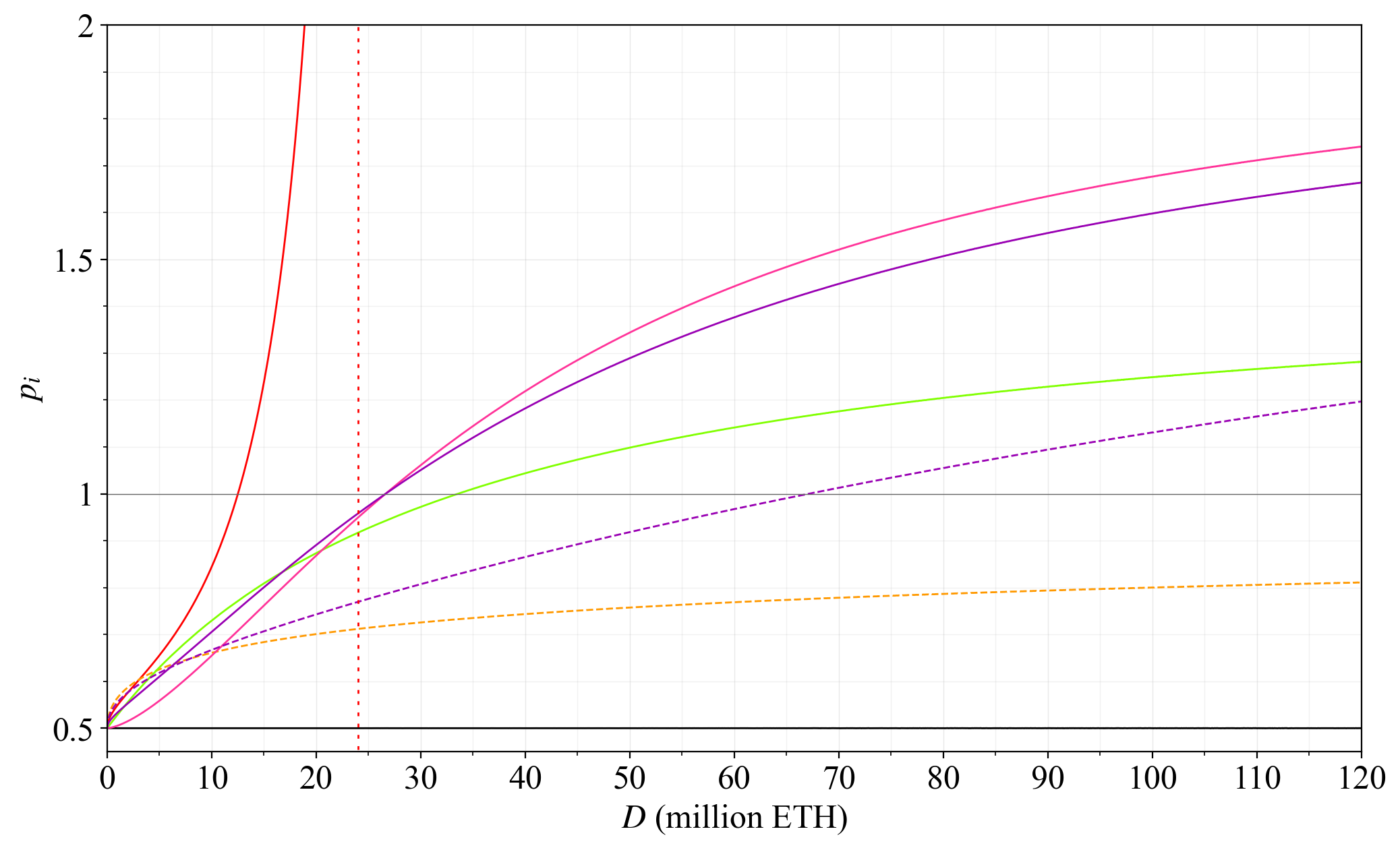
Figure 40. The negated inverse issuance-yield point-elasticity of demand (p_i) across D for various reward curves analyzed in this post. Lower is better, but staying rather close to 1 should be perfectly acceptable.
It may be easier to find agreement on something like the lime or dashed purple curve. A middle ground that can be implemented under rough consensus is better than the status quo. This includes a middle ground of simply adjusting the base reward factor, perhaps even higher than F=32, say to F=40. Such a change could still be helpful, with the understanding that MEV burn is still in the cards and will naturally affect staking rewards as well. It is also important to not be too rigid in assumptions around the supply curve and future REV at this point; it is not yet known how these economic forces will develop.
Pushing for the more ambitious reductions in issuance such as from the pink curve may not be worth it. Presumably, some members of the staking community will not be very welcoming to such changes (or any changes for that matter). It becomes a matter here of communicating the utility gains for Ethereum of adhering to MVI also under proof of stake. After all, stakers own the underlying ETH, and may reasonably hope that utility gains for Ethereum make its native token more attractive. A fruitful discussion within the Ethereum community and further research would at this point be very welcome.
Variability also depends on the frame of reference. Stakers may ultimately be more affected by fiat-denominated price fluctuations of the ETH token. The Sharp ratio, which is essentially the inverse of the RSD, would in reality be measured on a fiat basis today. But the relative frame of reference of keeping the analysis denominated in ETH is very helpful for clarifying how variables relate directly to each other. It isolates effects directly under a staker’s or developer’s control, which is important in staking economics.
5.5 Potential candidate for a new reward curve
Properties of a few different types of reward curves with various parameterizations have been presented. Among these, the R_{1.5} reward curve (lime in figures) with equation
using F=64 and k=2^{-25} will here be highlighted as a potential candidate if Ethereum updates the issuance policy. Its equation for issuance is
The candidate reward curve has been designed to provide very clear mental models related to the reference point D=2^{25} (around 33.6M ETH), that has been highlighted as a point below which it is desirable to keep the deposit size. Specifically, at D=2^{25}, the reward curve:
- Institutes an exact halving of issuance relative to the current reward curve (both y_i and Y_i). Each multiple of 2^{25}, gives a further reduction to 1/3 and 1/4 respectively.
- Reaches its peak issuance. If D>2^{25}, the issuance will begin to fall (naturally, the issuance yield will always fall with a rise in D).
- Lets the p_i-elasticity pass 1, and allows it to moderately rise with a rise in D.
- Lets the proportion of the yield assigned for attestations begin to fall, but keeps it roughly above 0.5 at the current level of REV and above 1/3 across the full range if the REV was to double. This is a compromise between safety and MVI that attempts to balance the situation before MEV burn.
- Lets the SSD begin to rise, but still ensures that it rises only moderately.
The reward curve also provides sufficient assurances of keeping D>14 M ETH, both before and after MEV burn is in place.
As a proof of (1), the candidate reward curve provides a fraction of the issuance yield of the current reward curve of
Since k=2^{-25}, kD becomes 1 at D=2^{25}, and 2 at D=2\times2^{25} etc.
To understand (2), first describe issuance as Y_i = \frac{cF}{1/\sqrt{D}+k\sqrt{D}}. The relevant critical point of the denominator can be determined by first computing its derivative
and finding where it equals zero by multiplication with the least common multiplier 2D^{3/2}. This gives
and thus the condition is D=1/k=2^{25}.
Note that (3) and (4) follow directly from 2. To summarize, the candidate reward curve offers a balanced compromise that preserves adequate consensus incentives while trying to push Ethereum toward MVI. There is also a clear rationale behind its parameterization, something that may make it easier to unite on.
6. Conclusion and discussion
The effect of issuance level on consensus incentives and reward variability was studied. When it comes to preserving correct consensus incentives, it is desirable to provide sufficient rewards to attesters relative to the rewards that proposers get, and to not let penalties become too low. Under the current reward scheme, this limits how much issuance can be reduced. Likewise, when considering reward variability for solo stakers, there are also good reasons to let issuance be a relevant proportion of all rewards, since it can be distributed with low variability.
It is important to recognize the need for formulating our issuance policy as derived from a set of tangible utility measures, providing a rationale for its implementation. Each deposit size can be assigned a maximum protocol utility issuance level. In the absence of a consensus redesign and/or introduction of a staking fee, that level is never too close to 0. But it is also important to not let issuance go above what is needed for retaining security—because that degrades utility for users. In a world without MEV or concern for the conditions of solo staking, designing our issuance policy would be a simpler affair. But MEV will imbalance consensus roles, produce variability, increase uncertainty and keep us from achieving MVI until we burn it. If we succeed in burning MEV, a staking fee discussed in Section 3 will presumably not be needed. If the endogenous yield is zero or negative, there are no direct incentives for staking. Implementing a staking fee at this point thus seems hard to motivate.
While the protocol could allow information about the implied supply curve to influence issuance in the future (i.e., autonomous adjustments), such practices are currently not very beneficial when contemplating our strict dependency on MEV. Still, the impetus for tempering our issuance policy should be clear from previous writings on MVI. It is of course not desirable to incentivize users to (delegate) stake when there is no need for it. If Ethereum should temper issuance, the available options can essentially be divided into the three categories presented in Table 2.
| Description | Analytical overview |
|---|---|
| A reduction of the base reward factor, keeping the current reward curve. | The change is minimal and easy to overview and implement. However, the current reward curve specifies an increasing issuance even as the deposit size rises far above what is needed for security, and therefore does not facilitate MVI. |
| A reward curve that approaches constant issuance. | Issuance is maintained at the same level relative to MEV, ceteris paribus. This keeps several important features rather neutral across D. Acts as a middle ground. |
| A reward curve where issuance falls moderately once past a desirable D. | We assert that allowing the deposit size to grow close to the maximum is so detrimental that we should not keep other features neutral. Issuance is thus allowed to fall moderately, but not to a level that jeopardizes consensus stability. |
Table 2. Main suggested options for potentially tempering issuance in Ethereum.
Section 5.5 suggested a viable candidate if the community decides that issuance should be tempered. It has a moderately falling issuance level as D increases past 2^{25}. Its equation is
with k=2^{-25} and F=64. This reward curve institutes an issuance halving relative to the current reward curve at D=2^{25}, and also lets issuance fall if D rises beyond that quantity of stake.
It would be beneficial and interesting to provide a more explicit utility mapping across deposit size and issuance yield, including a description of its computation. A rough reward curve could be discerned directly from such a map, which would be a nice way of visualizing the design. The parameterization of a reward curve could also be computed directly from such a utility map. Curve fittings involving 2-3 parameters have been sufficient for deriving a suitable curve in preliminary experimentation (for example using the Burr Type XII distribution). This would however represent a shift in design philosophy away from hand-crafted settings towards a data-driven approach. I come from the machine learning community, where the utility function generally takes a more central stage when designing and explaining a policy, rather than the specific weights or settings that ultimately are responsible for the supposed utility maximization. Fitted approaches will naturally lead to a higher accuracy when measured against the relevant utility function. It is at the same time true that a simple equation may make communication with a wider audience easier, and the candidate reward curve was designed with this in mind.
With a more restrictive issuance policy in place, such as something close to the reward curve suggested in Section 5.5, Ethereum would arguably find itself in a more favorable and balanced position, in particular after adopting MEV burn. The only other remaining near-term policy step (that can be implemented before MEV burn) is to let issuance vary with d instead of D for the adopted equation (h/t Buterin for discussion of a direct swap). The rationale was presented in my previous thread. This then brings us very close to letting the circulating supply drift (potentially perpetually deflate) under a dynamic equilibrium, something I hold as the optimal long-term vision for Ethereum’s issuance policy.